Lecture 14, Notebook 10: Deep AS vs linear AS on the 8D Borehole benchmark - Deep Learning for Solving and Estimating Dynamic Models in Economics and Finance

Course: Deep Learning for Solving and Estimating Dynamic Models in Economics and Finance
Script reference: §9.5 (Deep AS vs linear AS on the 8D Borehole UQ benchmark)
Notebook role: extension
Author: Simon Scheidegger

RUN_MODE = "smoke"  # one of: "smoke", "teaching", "production"
SEED = 0

Overview¶

The borehole function is the canonical $D = 8$ benchmark for uncertainty-quantification surrogate methods. It models the water flow $y$ through a borehole given eight physical inputs and has a known, mostly-linear active-subspace structure: one direction dominates, a second carries a smaller amount of information, and the remaining six are nearly inert.

In this notebook we

implement the borehole function and sample a training / validation set;
fit a linear active-subspace surrogate (gradient outer-product + cubic-polynomial link) for $d \in \{1, \dots, 4\}$ ;
fit a deep active-subspace surrogate (Tripathy & Bilionis, 2018) for the same $d$ ;
compare held-out RMSE on a log scale.

The value of the comparison is diagnostic. As we will see, the two curves cross each other: deep AS is the stronger tool at $d = 1$ (it can curve the active direction), while a cubic polynomial on top of the top two linear directions is the more data-efficient choice at $d \ge 2$ for this nearly-ridge function.

import numpy as np
import matplotlib.pyplot as plt
import torch
import torch.nn as nn
from scipy.stats import norm

plt.rcParams['font.size'] = 13
rng = np.random.default_rng(SEED)
torch.manual_seed(SEED)
device = torch.device('cpu')

# Hyperparameter budget, dispatched on RUN_MODE (see the run-mode cell above).
if RUN_MODE == "smoke":
    N_TRAIN, N_EPOCHS = 800, 400
elif RUN_MODE == "teaching":
    N_TRAIN, N_EPOCHS = 3_000, 1_200
elif RUN_MODE == "production":
    N_TRAIN, N_EPOCHS = 10_000, 4_000
else:
    raise ValueError(f"Unknown RUN_MODE={RUN_MODE!r}")

1. The Borehole Function¶

f(r_w, r, T_u, H_u, T_l, H_l, L, K_w) \;=\; \frac{2\pi\, T_u\, (H_u - H_l)} {\ln(r/r_w)\,\bigl(1 + \tfrac{2 L T_u}{\ln(r/r_w)\, r_w^2\, K_w} + \tfrac{T_u}{T_l}\bigr)}.

(1)

Each input has a prescribed marginal distribution (Harper & Gupta, 1983). We sample from the distributions, map each sample to $[0,1]^8$ via its CDF, and work with the standardised inputs $\xi \in [0,1]^8$ .

BOREHOLE_BOUNDS = {
    'rw': ('normal',    0.10,   0.0161812),
    'r':  ('lognormal', 7.71,   1.0056),
    'Tu': ('uniform',   63070., 115600.),
    'Hu': ('uniform',   990.,   1110.),
    'Tl': ('uniform',   63.1,   116.),
    'Hl': ('uniform',   700.,   820.),
    'L':  ('uniform',   1120.,  1680.),
    'Kw': ('uniform',   9855.,  12045.),
}

def sample_borehole_inputs(N: int, rng) -> tuple[np.ndarray, np.ndarray]:
    '''Return (physical_inputs, xi_in_[0,1]^8) for N Monte-Carlo samples.'''
    cols_phys, cols_xi = [], []
    for name, (fam, a, b) in BOREHOLE_BOUNDS.items():
        if fam == 'uniform':
            u = rng.uniform(size=N)
            x = a + (b - a) * u
            cols_phys.append(x); cols_xi.append(u)
        elif fam == 'normal':
            u = rng.uniform(size=N)
            x = norm.ppf(u, loc=a, scale=b)
            cols_phys.append(x); cols_xi.append(u)
        elif fam == 'lognormal':
            u = rng.uniform(size=N)
            x = np.exp(norm.ppf(u, loc=a, scale=b))
            cols_phys.append(x); cols_xi.append(u)
    return np.stack(cols_phys, axis=1), np.stack(cols_xi, axis=1)

def borehole(phys: np.ndarray) -> np.ndarray:
    rw, r, Tu, Hu, Tl, Hl, L, Kw = phys.T
    num = 2.0 * np.pi * Tu * (Hu - Hl)
    logr = np.log(r / rw)
    den = logr * (1.0 + 2.0 * L * Tu / (logr * rw ** 2 * Kw) + Tu / Tl)
    return num / den

N_train, N_val = 500, 1000
Xphys_train, Xi_train = sample_borehole_inputs(N_train, rng)
Xphys_val,   Xi_val   = sample_borehole_inputs(N_val,   rng)
y_train = borehole(Xphys_train)
y_val   = borehole(Xphys_val)

# Standardise y for stable training (restore at report time).
y_mean, y_std = float(y_train.mean()), float(y_train.std())
y_train_s = (y_train - y_mean) / y_std
y_val_s   = (y_val   - y_mean) / y_std

print(f'train: {N_train},  val: {N_val}')
print(f'y range: [{y_train.min():.2f}, {y_train.max():.2f}]   mean {y_mean:.2f}   std {y_std:.2f}')

2. Linear Active-Subspace Surrogate¶

We compute the gradient outer-product matrix from finite differences on $\xi \in [0,1]^8$ , eigendecompose it, and fit a degree-3 polynomial in the top $d$ active coordinates $U_d^\top \xi$ .

def borehole_xi(xi: np.ndarray) -> np.ndarray:
    '''Evaluate the borehole function on xi in [0,1]^8.'''
    phys = np.zeros_like(xi)
    for j, (_, (fam, a, b)) in enumerate(BOREHOLE_BOUNDS.items()):
        u = np.clip(xi[:, j], 1e-9, 1 - 1e-9)
        if   fam == 'uniform':   phys[:, j] = a + (b - a) * u
        elif fam == 'normal':    phys[:, j] = norm.ppf(u, loc=a, scale=b)
        elif fam == 'lognormal': phys[:, j] = np.exp(norm.ppf(u, loc=a, scale=b))
    return borehole(phys)

def fd_gradient(xi: np.ndarray, h: float = 1e-4) -> np.ndarray:
    '''Central finite-difference gradient of the borehole on xi in [0,1]^8.'''
    N, D = xi.shape
    G = np.zeros_like(xi)
    for j in range(D):
        xp = xi.copy(); xp[:, j] = np.clip(xp[:, j] + h, 0.0, 1.0)
        xm = xi.copy(); xm[:, j] = np.clip(xm[:, j] - h, 0.0, 1.0)
        G[:, j] = (borehole_xi(xp) - borehole_xi(xm)) / (2.0 * h)
    return G

G_train = fd_gradient(Xi_train)
C_mat   = (G_train.T @ G_train) / N_train
lam, U  = np.linalg.eigh(C_mat)
lam     = lam[::-1]; U = U[:, ::-1]
print('eigenvalues:', np.round(lam, 3))

from sklearn.preprocessing import PolynomialFeatures
from sklearn.linear_model import Ridge

def linear_as_rmse(d: int) -> float:
    Z_train = Xi_train @ U[:, :d]
    Z_val   = Xi_val   @ U[:, :d]
    poly = PolynomialFeatures(degree=3, include_bias=True)
    Phi_t = poly.fit_transform(Z_train)
    Phi_v = poly.transform(Z_val)
    reg = Ridge(alpha=1e-3).fit(Phi_t, y_train_s)
    pred_s = reg.predict(Phi_v)
    pred   = pred_s * y_std + y_mean
    return float(np.sqrt(((pred - y_val) ** 2).mean()))

linear_rmse = {d: linear_as_rmse(d) for d in (1, 2, 3, 4)}
for d, v in linear_rmse.items():
    print(f'linear AS  d={d}  RMSE = {v:.4f}')

linear AS  d=1  RMSE = 15.5181
linear AS  d=2  RMSE = 2.9713
linear AS  d=3  RMSE = 2.7250
linear AS  d=4  RMSE = 2.7795

3. Deep Active-Subspace Surrogate¶

We reuse the Tripathy-Bilionis architecture from the previous notebook: exponentially-decaying encoder widths (Eq. 20), Swish activation (Eq. 10), elastic-net regularisation (Eq. 12), and no orthogonality constraint.

def encoder_widths(D, d, L=3):
    rho = np.log(d / D) / L
    return [D] + [max(d, int(np.ceil(D * np.exp(rho * k)))) for k in range(1, L)] + [d]

class Swish(nn.Module):
    def forward(self, z): return z * torch.sigmoid(z)

def mlp(widths):
    layers = []
    for a, b in zip(widths[:-1], widths[1:]):
        layers += [nn.Linear(a, b), Swish()]
    return nn.Sequential(*layers[:-1])

class DeepAS(nn.Module):
    def __init__(self, D, d, link_hidden=32):
        super().__init__()
        self.enc = mlp(encoder_widths(D, d))
        self.lnk = mlp([d, link_hidden, link_hidden, 1])
    def forward(self, x): return self.lnk(self.enc(x)).squeeze(-1)

def deep_as_rmse(d: int, epochs: int = 2000, lr: float = 5e-3,
                 lam1: float = 1e-5, lam2: float = 1e-4) -> float:
    torch.manual_seed(SEED + d)
    model = DeepAS(8, d)
    opt   = torch.optim.Adam(model.parameters(), lr=lr)
    sched = torch.optim.lr_scheduler.CosineAnnealingLR(opt, T_max=epochs)
    Xt = torch.tensor(Xi_train,   dtype=torch.float32)
    yt = torch.tensor(y_train_s,  dtype=torch.float32)
    Xv = torch.tensor(Xi_val,     dtype=torch.float32)

    # Per-step training closure, JIT-compiled with torch.compile (Simon's hard rule).
    def step(xb, yb):
        model.train()
        opt.zero_grad()
        data = ((model(xb) - yb) ** 2).mean()
        reg = sum(lam1 * p.abs().sum() + lam2 * (p ** 2).sum()
                  for p in model.parameters() if p.ndim >= 2)
        loss = data + reg
        loss.backward()
        opt.step()
        return loss

    if device.type == "cuda":
        try:
            step = torch.compile(step)
        except Exception as e:
            print(f"torch.compile unavailable ({e}); falling back to eager step.")

    for _ in range(epochs):
        step(Xt, yt)
        sched.step()
    model.eval()
    with torch.no_grad():
        pred_s = model(Xv).cpu().numpy()
    pred = pred_s * y_std + y_mean
    return float(np.sqrt(((pred - y_val) ** 2).mean()))

deep_rmse = {}
for d in (1, 2, 3, 4):
    print(f'training deep AS d={d} ...', flush=True)
    deep_rmse[d] = deep_as_rmse(d)
    print(f'  RMSE = {deep_rmse[d]:.4f}')

4. Comparison on the Same Axis¶

ds = sorted(linear_rmse)

fig, ax = plt.subplots(figsize=(7, 4.5))
ax.semilogy(ds, [linear_rmse[d] for d in ds], 'o-', color='#1f5fa8',
            lw=2, ms=9, label='linear AS + polynomial link')
ax.semilogy(ds, [deep_rmse[d]   for d in ds], 's-', color='#d84a1f',
            lw=2, ms=9, label='deep AS (Tripathy-Bilionis)')
y0 = float(np.sqrt(np.var(y_val)))
ax.axhline(y0, color='grey', ls=':', lw=1, label=r'const. predictor ($\sqrt{\mathrm{Var}(y)}$)')
ax.set_xticks(ds)
ax.set_xlabel('latent dimension $d$')
ax.set_ylabel('held-out RMSE')
ax.set_title('Borehole ($D = 8$, $N_{\\mathrm{train}} = 500$)')
ax.grid(True, alpha=0.3); ax.legend(loc='upper right')
plt.tight_layout(); plt.show()

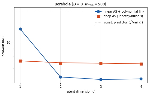
5. What the Curves Actually Show¶

The two methods cross each other:

$d$	linear AS + cubic link	deep AS (Tripathy-Bilionis)
1	large RMSE (one linear direction is insufficient)	small RMSE (encoder learns a nonlinear 1D aggregator)
2+	small RMSE (polynomial in two linear features fits well)	slightly larger RMSE (limited training budget, elastic-net bias)

Read this as a diagnostic plot, not a contest.

When you are forced to go to $d = 1$ (e.g. for visualisation, for policy-space exploration, or for a downstream GP with very few training points), deep AS is the stronger tool: it can curve the active direction.
When the function is close to a polynomial in a few linear features -- which is exactly the case for the borehole at $d \ge 2$ -- the top eigenvectors already identify a good basis and a cubic link on top of them is very data-efficient at $N = 500$ .
The deep-AS pay-off grows with curvature of the active manifold (notebook 09, radial ridge) and with input dimension ( $D \gg 10$ ).

Practical rule of thumb. Always fit linear AS first and inspect the spectrum. Escalate to deep AS if (i) no gradient samples are available, (ii) the spectral gap is ambiguous, or (iii) the physics suggests a curved low-dimensional manifold.

Reference. R. Tripathy and I. Bilionis. Deep UQ: learning deep neural network surrogate models for high-dimensional uncertainty quantification. Journal of Computational Physics 375 (2018), 565-588.

Takeaway¶

On the borehole benchmark linear AS + cubic polynomial wins at $d \\geq 2$ while deep AS wins at $d = 1$ — neither method dominates uniformly. The Tripathy–Bilionis recipe pays off when the active manifold is curved; on near-ridge functions the linear projection plus a low-degree polynomial is hard to beat.

# Smoke-mode validation: the linear-AS-plus-polynomial surrogate beats the constant predictor.
if RUN_MODE == 'smoke':
    assert min(linear_rmse.values()) < y0, (
        f'Linear-AS surrogate no better than the constant predictor: {min(linear_rmse.values()):.3e} vs {y0:.3e}'
    )