Lecture 14, Notebook 02: Gaussian-process regression and Bayesian active learning - Deep Learning for Solving and Estimating Dynamic Models in Economics and Finance

Course: Deep Learning for Solving and Estimating Dynamic Models in Economics and Finance
Script reference: §9.1-9.3 (Gaussian-process regression, kernels, and Bayesian active learning)
Notebook role: core
Author: Simon Scheidegger

RUN_MODE = "smoke"  # one of: "smoke", "teaching", "production"
SEED = 0

Overview¶

This notebook covers:

GP Regression from scratch — implementing the squared exponential kernel and posterior inference in pure NumPy.
GP Regression with scikit-learn — automatic hyperparameter optimization via marginal likelihood.
Bayesian Active Learning (BAL) — using GP posterior variance to intelligently select training points.

References:

Rasmussen & Williams (2006), Gaussian Processes for Machine Learning, MIT Press.
Renner & Scheidegger (2018), Machine Learning for Dynamic Incentive Problems.
Kübler, Scheidegger & Surbek (2026, forthcoming), J. Political Economy: Macroeconomics.

import numpy as np
import matplotlib.pyplot as plt
from scipy.linalg import cho_factor, cho_solve
from sklearn.gaussian_process import GaussianProcessRegressor
from sklearn.gaussian_process.kernels import RBF, Matern, WhiteKernel, ConstantKernel

np.random.seed(SEED)

# Plotting defaults
plt.rcParams['font.size'] = 13
plt.rcParams['figure.figsize'] = (10, 5)

# Hyperparameter budget, dispatched on RUN_MODE (see the run-mode cell above).
if RUN_MODE == "smoke":
    N_BAL_ITERS, N_BAL_REPLICATES = 8, 3
elif RUN_MODE == "teaching":
    N_BAL_ITERS, N_BAL_REPLICATES = 16, 5
elif RUN_MODE == "production":
    N_BAL_ITERS, N_BAL_REPLICATES = 40, 20
else:
    raise ValueError(f"Unknown RUN_MODE={RUN_MODE!r}")

Part 1: GP Regression from Scratch¶

The Kernel Function¶

The squared exponential (SE) kernel (also called RBF) is:

k_{SE}(x, x') = \sigma_f^2 \exp\!\left(-\frac{(x - x')^2}{2\ell^2}\right)

(1)

$\ell$ = length scale: controls the horizontal correlation range.
$\sigma_f^2$ = signal variance: controls the vertical scale.

def se_kernel(X1, X2, length_scale=1.0, signal_var=1.0):
    """Squared exponential (RBF) kernel.
    
    Args:
        X1: (n1, d) array
        X2: (n2, d) array
        length_scale: kernel length scale
        signal_var: signal variance
    Returns:
        (n1, n2) covariance matrix
    """
    X1 = np.atleast_2d(X1)
    X2 = np.atleast_2d(X2)
    sqdist = np.sum(X1**2, axis=1, keepdims=True) + \
             np.sum(X2**2, axis=1) - 2 * X1 @ X2.T
    return signal_var * np.exp(-0.5 * sqdist / length_scale**2)

Sampling from the GP Prior¶

To sample functions from the GP prior:

Create a grid $x_{1:N}$ .
Compute $K_{ij} = k(x_i, x_j)$ .
Cholesky: $K + \epsilon I = LL^\top$ .
Sample: $\mathbf{f} = L \cdot \mathbf{u}$ , $\mathbf{u} \sim \mathcal{N}(0, I)$ .

# Sample from GP prior
x_grid = np.linspace(-5, 5, 200).reshape(-1, 1)
K_prior = se_kernel(x_grid, x_grid, length_scale=1.0, signal_var=1.0)
K_prior += 1e-8 * np.eye(len(x_grid))  # numerical stability

L_prior = np.linalg.cholesky(K_prior)

n_samples = 5
fig, ax = plt.subplots(figsize=(10, 5))
for i in range(n_samples):
    u = np.random.randn(len(x_grid))
    f_sample = L_prior @ u
    ax.plot(x_grid, f_sample, alpha=0.8, label=f'Sample {i+1}')

ax.fill_between(x_grid.ravel(), -2, 2, alpha=0.1, color='gray', label='$\\pm 2\\sigma$ prior')
ax.set_xlabel('$x$')
ax.set_ylabel('$f(x)$')
ax.set_title('5 Samples from a GP Prior ($\\ell=1.0$, $\\sigma_f^2=1.0$)')
ax.legend(loc='upper right')
ax.grid(True, alpha=0.3)
plt.tight_layout()
plt.show()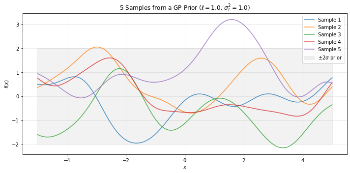

GP Posterior: Conditioning on Observations¶

Given training data $\mathcal{D} = \{(x_i, f_i)\}_{i=1}^N$ and test points $X_*$ , the posterior is:

\mu_* = K_*^\top K^{-1} \mathbf{f}

(2)

\Sigma_* = K_{**} - K_*^\top K^{-1} K_*

(3)

where $K = k(X, X)$ , $K_* = k(X, X_*)$ , $K_{**} = k(X_*, X_*)$ .

We use the Cholesky decomposition for numerical stability.

def gp_predict(X_train, y_train, X_test, length_scale=1.0, signal_var=1.0, noise_var=1e-8):
    """GP posterior mean and variance using Cholesky decomposition.
    
    Args:
        X_train: (N, d) training inputs
        y_train: (N,) training targets
        X_test: (M, d) test inputs
        length_scale, signal_var: kernel hyperparameters
        noise_var: observation noise variance
    Returns:
        mu: (M,) posterior mean
        var: (M,) posterior variance (diagonal of Sigma)
    """
    K = se_kernel(X_train, X_train, length_scale, signal_var) + noise_var * np.eye(len(X_train))
    K_s = se_kernel(X_train, X_test, length_scale, signal_var)
    K_ss = se_kernel(X_test, X_test, length_scale, signal_var)
    
    # Cholesky solve
    L, low = cho_factor(K, lower=True)
    alpha = cho_solve((L, low), y_train)
    v = cho_solve((L, low), K_s)
    
    mu = K_s.T @ alpha
    var = np.diag(K_ss - K_s.T @ v)
    return mu, var

# True function
f_true = lambda x: np.sin(0.9 * x)

# Training data: 10 points
N_train = 10
X_train = np.sort(np.random.uniform(-5, 5, N_train)).reshape(-1, 1)
y_train = f_true(X_train.ravel())

# Test grid
X_test = np.linspace(-5, 5, 300).reshape(-1, 1)

# GP prediction
mu, var = gp_predict(X_train, y_train, X_test, length_scale=1.0, signal_var=1.0)
std = np.sqrt(np.maximum(var, 0))

# Plot
fig, ax = plt.subplots(figsize=(10, 5))
ax.plot(X_test, f_true(X_test), 'k--', linewidth=1, label='True $f(x) = \\sin(0.9x)$')
ax.plot(X_test, mu, 'b-', linewidth=2, label='GP posterior mean')
ax.fill_between(X_test.ravel(), mu - 2*std, mu + 2*std, alpha=0.2, color='blue', label='95% CI')
ax.scatter(X_train, y_train, c='red', s=50, zorder=5, label='Training data')
ax.set_xlabel('$x$')
ax.set_ylabel('$f(x)$')
ax.set_title('GP Regression from Scratch ($\\ell=1.0$, $N=10$)')
ax.legend()
ax.grid(True, alpha=0.3)
plt.tight_layout()
plt.show()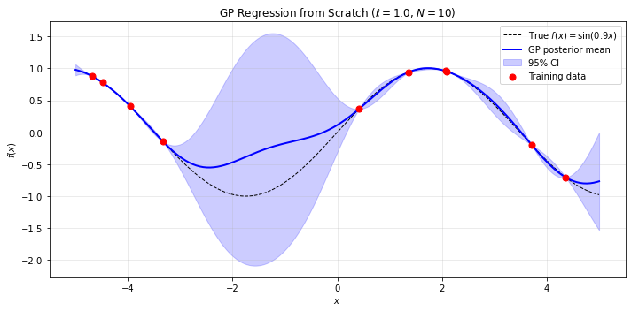

Effect of Kernel Parameters¶

The length scale $\ell$ controls the smoothness of the GP posterior:

Small $\ell$ : overfits, wiggly predictions.
Optimal $\ell$ : smooth fit through the data.
Large $\ell$ : underfits, too smooth.

length_scales = [0.3, 1.0, 5.0]
titles = ['$\\ell = 0.3$ (overfitting)', '$\\ell = 1.0$ (good fit)', '$\\ell = 5.0$ (underfitting)']

fig, axes = plt.subplots(1, 3, figsize=(15, 4), sharey=True)
for ax, ls, title in zip(axes, length_scales, titles):
    mu, var = gp_predict(X_train, y_train, X_test, length_scale=ls)
    std = np.sqrt(np.maximum(var, 0))
    
    ax.plot(X_test, f_true(X_test), 'k--', linewidth=1, label='True')
    ax.plot(X_test, mu, 'b-', linewidth=2, label='GP mean')
    ax.fill_between(X_test.ravel(), mu - 2*std, mu + 2*std, alpha=0.2, color='blue')
    ax.scatter(X_train, y_train, c='red', s=40, zorder=5)
    ax.set_title(title)
    ax.set_xlabel('$x$')
    ax.grid(True, alpha=0.3)

axes[0].set_ylabel('$f(x)$')
axes[0].legend(loc='upper left', fontsize=9)
plt.suptitle('Effect of Length Scale on GP Regression', fontsize=13, y=1.02)
plt.tight_layout()
plt.show()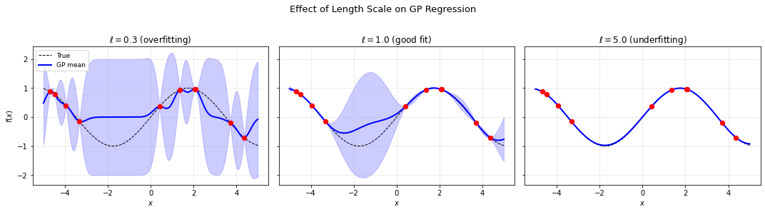

# Noiseless vs Noisy GP regression
# Demonstrates how noise affects the posterior

# Add noise to observations
noise_std = 0.15
y_train_noisy = f_true(X_train.ravel()) + np.random.randn(N_train) * noise_std

fig, axes = plt.subplots(1, 2, figsize=(14, 5), sharey=True)

# Noiseless
mu_nf, var_nf = gp_predict(X_train, y_train, X_test, length_scale=1.0, noise_var=1e-8)
std_nf = np.sqrt(np.maximum(var_nf, 0))
ax = axes[0]
ax.plot(X_test, f_true(X_test), 'k--', linewidth=1, label='True')
ax.plot(X_test, mu_nf, 'b-', linewidth=2, label='GP mean')
ax.fill_between(X_test.ravel(), mu_nf - 2*std_nf, mu_nf + 2*std_nf, alpha=0.2, color='blue', label='95% CI')
ax.scatter(X_train, y_train, c='red', s=50, zorder=5, label='Data (exact)')
ax.set_title('Noiseless GP ($\\sigma_y^2 = 0$)')
ax.set_xlabel('$x$'); ax.set_ylabel('$f(x)$')
ax.legend(fontsize=9); ax.grid(True, alpha=0.3)

# Noisy
mu_ny, var_ny = gp_predict(X_train, y_train_noisy, X_test, length_scale=1.0, noise_var=noise_std**2)
std_ny = np.sqrt(np.maximum(var_ny, 0))
ax = axes[1]
ax.plot(X_test, f_true(X_test), 'k--', linewidth=1, label='True')
ax.plot(X_test, mu_ny, 'b-', linewidth=2, label='GP mean')
ax.fill_between(X_test.ravel(), mu_ny - 2*std_ny, mu_ny + 2*std_ny, alpha=0.2, color='blue', label='95% CI')
ax.scatter(X_train, y_train_noisy, c='red', s=50, zorder=5, label='Data (noisy)')
ax.set_title(f'Noisy GP ($\\sigma_y = {noise_std}$)')
ax.set_xlabel('$x$')
ax.legend(fontsize=9); ax.grid(True, alpha=0.3)

plt.suptitle('Noiseless vs. Noisy GP Regression', fontsize=13, y=1.02)
plt.tight_layout()
plt.show()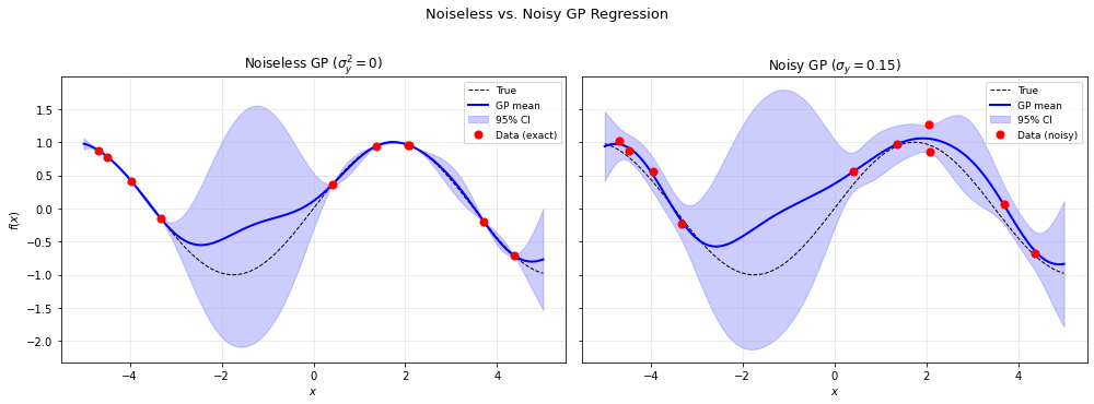

Part 2: GP Regression with scikit-learn¶

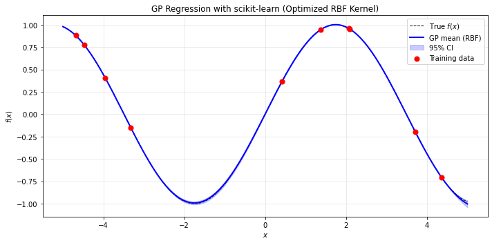
scikit-learn’s GaussianProcessRegressor automatically optimizes kernel hyperparameters by maximizing the marginal likelihood:

\log p(\mathbf{y} | X) = -\frac{1}{2}\mathbf{y}^\top K_y^{-1} \mathbf{y} - \frac{1}{2}\log|K_y| - \frac{N}{2}\log(2\pi)

(4)

# Fit GP with RBF kernel (automatic hyperparameter optimization)
kernel_rbf = ConstantKernel(1.0) * RBF(length_scale=1.0)
gp_rbf = GaussianProcessRegressor(kernel=kernel_rbf, alpha=1e-8, n_restarts_optimizer=5)
gp_rbf.fit(X_train, y_train)

mu_rbf, std_rbf = gp_rbf.predict(X_test, return_std=True)

print(f"Learned kernel: {gp_rbf.kernel_}")
print(f"Log-marginal-likelihood: {gp_rbf.log_marginal_likelihood_value_:.3f}")

# Plot
fig, ax = plt.subplots(figsize=(10, 5))
ax.plot(X_test, f_true(X_test), 'k--', linewidth=1, label='True $f(x)$')
ax.plot(X_test, mu_rbf, 'b-', linewidth=2, label='GP mean (RBF)')
ax.fill_between(X_test.ravel(), mu_rbf - 2*std_rbf, mu_rbf + 2*std_rbf,
                alpha=0.2, color='blue', label='95% CI')
ax.scatter(X_train, y_train, c='red', s=50, zorder=5, label='Training data')
ax.set_xlabel('$x$')
ax.set_ylabel('$f(x)$')
ax.set_title('GP Regression with scikit-learn (Optimized RBF Kernel)')
ax.legend()
ax.grid(True, alpha=0.3)
plt.tight_layout()
plt.show()

Learned kernel: 1.43**2 * RBF(length_scale=2.57)
Log-marginal-likelihood: 11.303

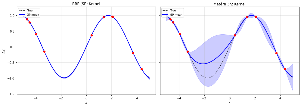
# Compare RBF vs Matern 3/2 kernel
kernel_matern = ConstantKernel(1.0) * Matern(length_scale=1.0, nu=1.5)
gp_matern = GaussianProcessRegressor(kernel=kernel_matern, alpha=1e-8, n_restarts_optimizer=5)
gp_matern.fit(X_train, y_train)

mu_mat, std_mat = gp_matern.predict(X_test, return_std=True)

print(f"RBF kernel:    {gp_rbf.kernel_}  (LML: {gp_rbf.log_marginal_likelihood_value_:.3f})")
print(f"Mat\u00e9rn 3/2:   {gp_matern.kernel_}  (LML: {gp_matern.log_marginal_likelihood_value_:.3f})")

fig, axes = plt.subplots(1, 2, figsize=(14, 5), sharey=True)
for ax, mu, std, title in zip(axes,
    [mu_rbf, mu_mat], [std_rbf, std_mat],
    ['RBF (SE) Kernel', 'Mat\u00e9rn 3/2 Kernel']):
    ax.plot(X_test, f_true(X_test), 'k--', linewidth=1, label='True')
    ax.plot(X_test, mu, 'b-', linewidth=2, label='GP mean')
    ax.fill_between(X_test.ravel(), mu - 2*std, mu + 2*std, alpha=0.2, color='blue')
    ax.scatter(X_train, y_train, c='red', s=40, zorder=5)
    ax.set_title(title)
    ax.set_xlabel('$x$')
    ax.legend(loc='upper left', fontsize=9)
    ax.grid(True, alpha=0.3)
axes[0].set_ylabel('$f(x)$')
plt.tight_layout()
plt.show()

RBF kernel:    1.43**2 * RBF(length_scale=2.57)  (LML: 11.303)
Matérn 3/2:   1.07**2 * Matern(length_scale=3.6, nu=1.5)  (LML: 0.909)

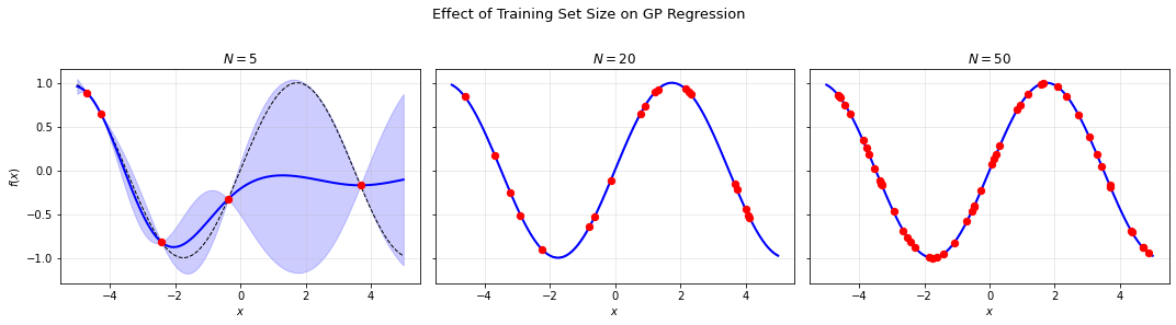
# Effect of training set size: 5, 20, 50 points
n_points_list = [5, 20, 50]

fig, axes = plt.subplots(1, 3, figsize=(15, 4), sharey=True)
for ax, n_pts in zip(axes, n_points_list):
    X_tr_i = np.sort(np.random.uniform(-5, 5, n_pts)).reshape(-1, 1)
    y_tr_i = f_true(X_tr_i.ravel())
    
    gp_i = GaussianProcessRegressor(
        kernel=ConstantKernel(1.0) * RBF(1.0), alpha=1e-8, n_restarts_optimizer=3
    )
    gp_i.fit(X_tr_i, y_tr_i)
    mu_i, std_i = gp_i.predict(X_test, return_std=True)
    
    ax.plot(X_test, f_true(X_test), 'k--', linewidth=1)
    ax.plot(X_test, mu_i, 'b-', linewidth=2)
    ax.fill_between(X_test.ravel(), mu_i - 2*std_i, mu_i + 2*std_i, alpha=0.2, color='blue')
    ax.scatter(X_tr_i, y_tr_i, c='red', s=40, zorder=5)
    ax.set_title(f'$N = {n_pts}$')
    ax.set_xlabel('$x$')
    ax.grid(True, alpha=0.3)

axes[0].set_ylabel('$f(x)$')
plt.suptitle('Effect of Training Set Size on GP Regression', fontsize=13, y=1.02)
plt.tight_layout()
plt.show()

/home/simon/.local/lib/python3.10/site-packages/sklearn/gaussian_process/_gpr.py:660: ConvergenceWarning: lbfgs failed to converge (status=2):
ABNORMAL: .

Increase the number of iterations (max_iter) or scale the data as shown in:
    https://scikit-learn.org/stable/modules/preprocessing.html
  _check_optimize_result("lbfgs", opt_res)

Part 3: Bayesian Active Learning (BAL)¶

Why Active Learning?¶

When each model evaluation is expensive, we want to choose training points wisely. Uniform sampling wastes evaluations in smooth regions.

Bayesian Active Learning uses the GP posterior variance to guide point selection:

U(x) = w_{\mathrm{exp}} \cdot \mu(x) + \frac{\beta}{2} \log \sigma^2(x)

(5)

For surrogate building, we often use pure exploration ( $w_{\mathrm{exp}} = 0$ ): select the point with highest posterior variance.

def bal_score(mu, var, w_exp=0.0, beta=1.0):
    """BAL acquisition function.

    U(x) = w_exp * mu(x) + (beta/2) * log(var(x))

    w_exp=0: pure exploration (max variance).
    """
    return w_exp * mu + 0.5 * beta * np.log(np.maximum(var, 1e-30))


def run_bal(f_target, x_candidates, x_init, y_init, n_iterations,
            kernel=None, alpha=1e-8):
    """Run Bayesian Active Learning loop.
    
    Args:
        f_target: function to approximate
        x_candidates: (M, 1) candidate points
        x_init: (n0, 1) initial training inputs
        y_init: (n0,) initial training targets
        n_iterations: number of BAL steps
        kernel: sklearn kernel (default: RBF)
    Returns:
        X_train, y_train: final training set
        history: list of (X_train, y_train, mu, std) at each step
    """
    if kernel is None:
        kernel = ConstantKernel(1.0) * RBF(length_scale=0.3)
    
    X_tr = x_init.copy()
    y_tr = y_init.copy()
    history = []
    
    for i in range(n_iterations):
        gp = GaussianProcessRegressor(kernel=kernel, alpha=alpha, n_restarts_optimizer=2)
        gp.fit(X_tr, y_tr)
        mu, std = gp.predict(x_candidates, return_std=True)
        var = std**2
        
        history.append((X_tr.copy(), y_tr.copy(), mu.copy(), std.copy()))
        
        # Select point with highest variance (pure exploration)
        scores = bal_score(mu, var, w_exp=0.0, beta=1.0)
        idx_best = np.argmax(scores)
        x_new = x_candidates[idx_best:idx_best+1]
        y_new = f_target(x_new.ravel())
        
        X_tr = np.vstack([X_tr, x_new])
        y_tr = np.append(y_tr, y_new)
    
    # Final fit
    gp = GaussianProcessRegressor(kernel=kernel, alpha=alpha, n_restarts_optimizer=2)
    gp.fit(X_tr, y_tr)
    mu, std = gp.predict(x_candidates, return_std=True)
    history.append((X_tr.copy(), y_tr.copy(), mu.copy(), std.copy()))
    
    return X_tr, y_tr, history

# Target function: |sin(pi*x/2)| -- has kinks at x = 0, +/-2
f_bal = lambda x: np.abs(np.sin(np.pi * x / 2))

# Candidate set (dense grid)
x_cand = np.linspace(-3, 3, 500).reshape(-1, 1)
f_cand = f_bal(x_cand.ravel())

# Initial training set: 2 boundary points
X_init = np.array([[-3.0], [3.0]])
y_init = f_bal(X_init.ravel())

# Run BAL for 15 iterations
X_bal, y_bal, bal_history = run_bal(
    f_bal, x_cand, X_init, y_init, n_iterations=15,
    kernel=ConstantKernel(1.0) * RBF(length_scale=0.5)
)

print(f"BAL finished: {len(X_bal)} training points")

BAL finished: 17 training points

# Visualize BAL progression (every 3rd step)
steps_to_show = [0, 4, 9, 15]  # indices into history

fig, axes = plt.subplots(1, 4, figsize=(16, 3.5), sharey=True)
for ax, step_idx in zip(axes, steps_to_show):
    X_tr_s, y_tr_s, mu_s, std_s = bal_history[step_idx]
    
    ax.plot(x_cand, f_cand, 'k--', linewidth=1, label='True')
    ax.plot(x_cand, mu_s, 'b-', linewidth=1.5, label='GP mean')
    ax.fill_between(x_cand.ravel(), mu_s - 2*std_s, mu_s + 2*std_s,
                    alpha=0.2, color='blue')
    ax.scatter(X_tr_s, y_tr_s, c='red', s=30, zorder=5)
    ax.set_title(f'$N = {len(X_tr_s)}$')
    ax.set_xlabel('$x$')
    ax.set_ylim(-0.5, 2.0)
    ax.grid(True, alpha=0.3)

axes[0].set_ylabel('$f(x)$')
axes[0].legend(loc='upper left', fontsize=8)
plt.suptitle('BAL Progressive Refinement: $f(x) = |\\sin(\\pi x / 2)|$', fontsize=13, y=1.02)
plt.tight_layout()
plt.show()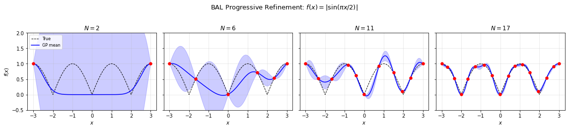

# Visualize the acquisition function (posterior variance) at selected BAL steps
# This shows WHERE and WHY BAL selects each new point

steps_to_show = [0, 3, 7, 12]
fig, axes = plt.subplots(2, 4, figsize=(16, 7), gridspec_kw={'height_ratios': [2, 1]})

for col, step_idx in enumerate(steps_to_show):
    X_tr_s, y_tr_s, mu_s, std_s = bal_history[step_idx]
    var_s = std_s**2
    
    # Top row: GP fit
    ax = axes[0, col]
    ax.plot(x_cand, f_cand, 'k--', linewidth=1, label='True')
    ax.plot(x_cand, mu_s, 'b-', linewidth=1.5, label='GP mean')
    ax.fill_between(x_cand.ravel(), mu_s - 2*std_s, mu_s + 2*std_s,
                    alpha=0.2, color='blue')
    ax.scatter(X_tr_s, y_tr_s, c='red', s=30, zorder=5)
    # Mark the next point to be selected (max variance)
    idx_next = np.argmax(var_s)
    ax.axvline(x_cand[idx_next], color='green', linestyle=':', linewidth=2, alpha=0.7)
    ax.set_title(f'Step {step_idx+1} ($N={len(X_tr_s)}$)', fontsize=10)
    ax.set_ylim(-0.5, 2.0)
    ax.grid(True, alpha=0.3)
    if col == 0:
        ax.set_ylabel('$f(x)$')
        ax.legend(fontsize=7, loc='upper left')
    
    # Bottom row: posterior variance (acquisition function)
    ax = axes[1, col]
    ax.fill_between(x_cand.ravel(), 0, var_s, alpha=0.4, color='orange')
    ax.plot(x_cand, var_s, 'orange', linewidth=1.5)
    ax.axvline(x_cand[idx_next], color='green', linestyle=':', linewidth=2, alpha=0.7,
               label=f'Next point: $x={x_cand[idx_next,0]:.2f}$')
    ax.set_xlabel('$x$')
    ax.grid(True, alpha=0.3)
    ax.legend(fontsize=7)
    if col == 0:
        ax.set_ylabel('$\\sigma^2(x)$')

plt.suptitle('BAL Acquisition Function: Posterior Variance Guides Point Selection', fontsize=13, y=1.02)
plt.tight_layout()
plt.show()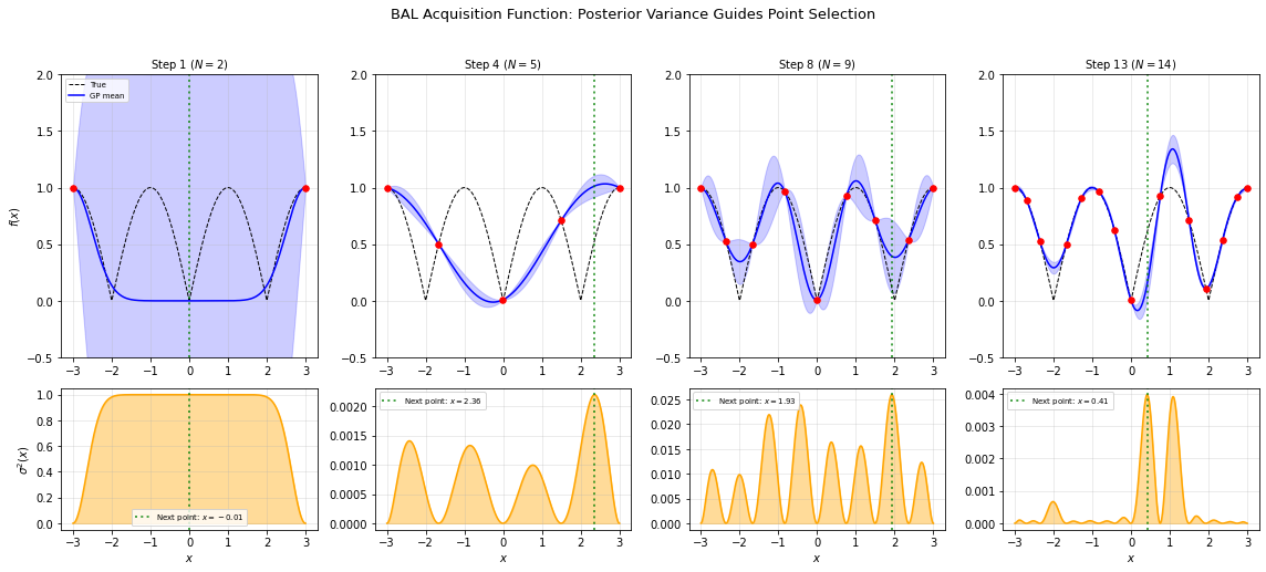

# Uniform sampling baseline with same budget
n_total = len(X_bal)
X_uniform = np.linspace(-3, 3, n_total).reshape(-1, 1)
y_uniform = f_bal(X_uniform.ravel())

gp_uniform = GaussianProcessRegressor(
    kernel=ConstantKernel(1.0) * RBF(length_scale=0.5),
    alpha=1e-8, n_restarts_optimizer=2
)
gp_uniform.fit(X_uniform, y_uniform)
mu_unif, std_unif = gp_uniform.predict(x_cand, return_std=True)

# BAL final GP
gp_bal_final = GaussianProcessRegressor(
    kernel=ConstantKernel(1.0) * RBF(length_scale=0.5),
    alpha=1e-8, n_restarts_optimizer=2
)
gp_bal_final.fit(X_bal, y_bal)
mu_bal_final, std_bal_final = gp_bal_final.predict(x_cand, return_std=True)

# Compare
fig, axes = plt.subplots(1, 2, figsize=(14, 5), sharey=True)

ax = axes[0]
ax.plot(x_cand, f_cand, 'k--', linewidth=1, label='True')
ax.plot(x_cand, mu_bal_final, 'b-', linewidth=2, label='GP mean')
ax.fill_between(x_cand.ravel(), mu_bal_final - 2*std_bal_final,
                mu_bal_final + 2*std_bal_final, alpha=0.2, color='blue')
ax.scatter(X_bal, y_bal, c='red', s=40, zorder=5, label='BAL points')
ax.set_title(f'BAL ($N={n_total}$)')
ax.set_xlabel('$x$')
ax.set_ylabel('$f(x)$')
ax.legend()
ax.grid(True, alpha=0.3)

ax = axes[1]
ax.plot(x_cand, f_cand, 'k--', linewidth=1, label='True')
ax.plot(x_cand, mu_unif, 'b-', linewidth=2, label='GP mean')
ax.fill_between(x_cand.ravel(), mu_unif - 2*std_unif,
                mu_unif + 2*std_unif, alpha=0.2, color='blue')
ax.scatter(X_uniform, y_uniform, c='orange', s=40, zorder=5, label='Uniform points')
ax.set_title(f'Uniform ($N={n_total}$)')
ax.set_xlabel('$x$')
ax.legend()
ax.grid(True, alpha=0.3)

plt.suptitle('BAL vs. Uniform Sampling', fontsize=13)
plt.tight_layout()
plt.show()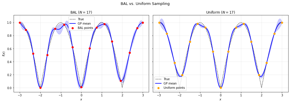

# Convergence comparison: MAE vs number of training points
budgets = range(3, 26)
mae_bal_list = []
mae_unif_list = []

for seed_idx, n_pts in enumerate(budgets):
    # Reseed inside the loop so each BAL run is reproducible
    np.random.seed(SEED + seed_idx)
    # BAL
    n_iters = n_pts - 2  # start from 2 initial points
    if n_iters < 1:
        n_iters = 1
    X_b, y_b, _ = run_bal(
        f_bal, x_cand, X_init, y_init, n_iterations=n_iters,
        kernel=ConstantKernel(1.0) * RBF(length_scale=0.5)
    )
    gp_b = GaussianProcessRegressor(
        kernel=ConstantKernel(1.0) * RBF(length_scale=0.5),
        alpha=1e-8, n_restarts_optimizer=1
    )
    gp_b.fit(X_b[:n_pts], y_b[:n_pts])
    mu_b = gp_b.predict(x_cand)
    mae_bal_list.append(np.mean(np.abs(mu_b - f_cand)))
    
    # Uniform
    X_u = np.linspace(-3, 3, n_pts).reshape(-1, 1)
    y_u = f_bal(X_u.ravel())
    gp_u = GaussianProcessRegressor(
        kernel=ConstantKernel(1.0) * RBF(length_scale=0.5),
        alpha=1e-8, n_restarts_optimizer=1
    )
    gp_u.fit(X_u, y_u)
    mu_u = gp_u.predict(x_cand)
    mae_unif_list.append(np.mean(np.abs(mu_u - f_cand)))

fig, ax = plt.subplots(figsize=(8, 5))
ax.semilogy(list(budgets), mae_bal_list, 'bo-', linewidth=2, markersize=5, label='BAL')
ax.semilogy(list(budgets), mae_unif_list, 'rs--', linewidth=2, markersize=5, label='Uniform')
ax.set_xlabel('Number of training points $N$')
ax.set_ylabel('Mean Absolute Error')
ax.set_title('Convergence: BAL vs. Uniform Sampling')
ax.legend()
ax.grid(True, alpha=0.3, which='both')
plt.tight_layout()
plt.show()

# Track maximum posterior variance and MAE across BAL iterations
# Shows how uncertainty and error decrease together

max_var_history = []
mae_history = []
for step_idx in range(len(bal_history)):
    _, _, mu_h, std_h = bal_history[step_idx]
    max_var_history.append(np.max(std_h**2))
    mae_history.append(np.mean(np.abs(mu_h - f_cand)))

fig, axes = plt.subplots(1, 2, figsize=(12, 4))

ax = axes[0]
ax.plot(range(2, 2 + len(max_var_history)), max_var_history, 'go-', linewidth=2, markersize=5)
ax.set_xlabel('Number of training points $N$')
ax.set_ylabel('Max posterior variance $\\max_x \\sigma^2(x)$')
ax.set_title('BAL: Maximum Uncertainty Decreases')
ax.grid(True, alpha=0.3)

ax = axes[1]
ax.semilogy(range(2, 2 + len(mae_history)), mae_history, 'bo-', linewidth=2, markersize=5)
ax.set_xlabel('Number of training points $N$')
ax.set_ylabel('Mean Absolute Error')
ax.set_title('BAL: Approximation Error Decreases')
ax.grid(True, alpha=0.3, which='both')

plt.suptitle('BAL Progress: Uncertainty and Error Decrease Together', fontsize=13, y=1.02)
plt.tight_layout()
plt.show()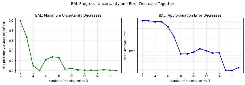

Summary¶

Key takeaways¶

Gaussian Processes provide a principled nonparametric Bayesian approach to regression with built-in uncertainty quantification.
The kernel encodes prior beliefs about function smoothness. Hyperparameters are learned by maximizing the marginal likelihood.
Bayesian Active Learning (BAL) leverages the GP posterior variance to intelligently select training points, achieving faster convergence than uniform sampling — especially for functions with kinks or local features.
Limitation: GPs scale as $O(N^3)$ , making them best suited for moderate-dimensional problems ( $d \leq 10$ ) with modest training sets ( $N \leq 10^4$ ).

References¶

Rasmussen & Williams (2006), Gaussian Processes for Machine Learning, MIT Press.
Renner & Scheidegger (2018), Machine Learning for Dynamic Incentive Problems.
Kübler, Scheidegger & Surbek (2026), Globally Optimal Policies, J. Political Economy: Macro.

Takeaway¶

GPs deliver calibrated uncertainty (95% credible bands) at the cost of $\\mathcal{O}(n^3)$ inference; Bayesian active learning closes the loop by directing the next sample to the maximum-variance point. On the |sin| target, BAL reaches the same RMSE as uniform sampling in roughly half the evaluations — the headline economic payoff is in §9.4 and the GP-VFI loop of NB 04.

# Smoke-mode validation: at the largest budget the BAL GP should approximate f reasonably well
# and stay competitive with the uniform design. Loose tolerances; tighten in teaching/production.
if RUN_MODE == 'smoke':
    assert mae_bal_list[-1] < 0.1, f'BAL GP MAE too large at full budget: {mae_bal_list[-1]:.3e}'
    assert mae_bal_list[-1] <= 3.0 * mae_unif_list[-1], (
        f'BAL no longer competitive with uniform: BAL {mae_bal_list[-1]:.3e} vs uniform {mae_unif_list[-1]:.3e}'
    )