Lecture 14, Notebook 09: Deep active subspaces — Tripathy & Bilionis on a 20D radial ridge - Deep Learning for Solving and Estimating Dynamic Models in Economics and Finance

Course: Deep Learning for Solving and Estimating Dynamic Models in Economics and Finance
Script reference: §9.5 (Deep active subspaces — Tripathy & Bilionis 2018 on a 20D radial-ridge function)
Notebook role: extension
Author: Simon Scheidegger

RUN_MODE = "smoke"  # one of: "smoke", "teaching", "production"
SEED = 0

Overview¶

The linear active-subspace (AS) method approximates a scalar map $f : \mathbb{R}^D \to \mathbb{R}$ as

f(\xi) \;\approx\; g\big(U_m^\top \xi\big), \qquad U_m \in \mathbb{R}^{D \times d},

(1)

i.e. a function of $d \ll D$ linear projections of the inputs. The matrix $U_m$ is the span of the top eigenvectors of the gradient outer-product matrix $C = \mathbb{E}[\nabla f \nabla f^\top]$ .

Failure mode. If the function varies along a curved manifold, linear projections cannot capture the low intrinsic dimension and one needs many components to represent the map accurately.

Fix (Tripathy & Bilionis, 2018). Replace the linear encoder with a deep neural network,

\hat f(\xi) \;=\; g\big(h(\xi)\big), \qquad h : \mathbb{R}^D \to \mathbb{R}^d, \quad g : \mathbb{R}^d \to \mathbb{R},

(2)

train $h$ and $g$ jointly by minimising the data loss plus an elastic-net penalty, and choose $d$ from the validation-MSE elbow. No gradient samples or Stiefel-manifold constraint are required.

What this notebook does.

Defines a radial-ridge target $y(\xi) = \exp\big(-[(w_1^\top\xi)^2 + (w_2^\top\xi)^2]\big)$ in $D = 20$ input dimensions.
Shows that linear AS needs $d_{\text{lin}} = 2$ active directions.
Trains a deep AS surrogate for $d \in \{1, 2, 3, 4\}$ and recovers the true intrinsic dimension $d_{\text{nl}} = 1$ from the validation-MSE elbow.
Visualises the learned 1D latent coordinate against the true radius $r^2 = (w_1^\top\xi)^2 + (w_2^\top\xi)^2$ .

import numpy as np
import matplotlib.pyplot as plt
import torch
import torch.nn as nn

plt.rcParams['font.size'] = 13
rng = np.random.default_rng(SEED)
torch.manual_seed(SEED)
device = torch.device("cuda" if torch.cuda.is_available() else "cpu")

# Hyperparameter budget, dispatched on RUN_MODE (see the run-mode cell above).
if RUN_MODE == "smoke":
    N_TRAIN, N_EPOCHS = 1_000, 400
elif RUN_MODE == "teaching":
    N_TRAIN, N_EPOCHS = 4_000, 1_200
elif RUN_MODE == "production":
    N_TRAIN, N_EPOCHS = 16_000, 4_000
else:
    raise ValueError(f"Unknown RUN_MODE={RUN_MODE!r}")

1. The Radial-Ridge Target¶

We pick two fixed unit vectors $w_1, w_2 \in \mathbb{R}^{20}$ with $w_1 \perp w_2$ and define

y(\xi) \;=\; \exp\!\Big( -\big[(w_1^\top \xi)^2 + (w_2^\top \xi)^2\big] \Big), \qquad \xi \sim \mathcal{N}(0, I_{20}).

(3)

The aggregator $r^2 = (w_1^\top\xi)^2 + (w_2^\top\xi)^2$ is a nonlinear function of two linear features, so

the linear AS sees two relevant directions ( $d_{\text{lin}} = 2$ );
a nonlinear encoder can collapse them into a single scalar ( $d_{\text{nl}} = 1$ ).

D = 20
# Two orthogonal unit directions in R^20.
W = rng.normal(size=(D, 2))
W, _ = np.linalg.qr(W)            # W has orthonormal columns
w1, w2 = W[:, 0], W[:, 1]

def target(Xi: np.ndarray) -> np.ndarray:
    s1 = Xi @ w1
    s2 = Xi @ w2
    return np.exp(-(s1 ** 2 + s2 ** 2))

def grad_target(Xi: np.ndarray) -> np.ndarray:
    s1 = (Xi @ w1)[:, None]
    s2 = (Xi @ w2)[:, None]
    fval = np.exp(-(s1 ** 2 + s2 ** 2))
    return -2.0 * fval * (s1 * w1 + s2 * w2)

N_train, N_val = 4000, 2000
Xi_train = rng.normal(size=(N_train, D))
Xi_val   = rng.normal(size=(N_val, D))
y_train  = target(Xi_train)
y_val    = target(Xi_val)

print(f"train set: Xi_train {Xi_train.shape}, y range [{y_train.min():.3f}, {y_train.max():.3f}]")

train set: Xi_train (4000, 20), y range [0.000, 0.999]

2. Linear Active Subspace Baseline¶

We form the gradient outer-product matrix

C \;=\; \tfrac{1}{N} \sum_{i=1}^N \nabla y(\xi_i)\, \nabla y(\xi_i)^\top

(4)

and inspect its spectrum. By construction only $w_1$ and $w_2$ carry information, so $C$ should have rank 2: a linear surrogate needs $d_{\text{lin}} = 2$ .

G = grad_target(Xi_train)            # (N, D)
C = (G.T @ G) / N_train              # (D, D)
eigvals, eigvecs = np.linalg.eigh(C)
eigvals = eigvals[::-1]              # descending
eigvecs = eigvecs[:, ::-1]

fig, ax = plt.subplots(figsize=(6, 4))
ax.semilogy(np.arange(1, D + 1), np.clip(eigvals, 1e-16, None), 'o-', color='#1f5fa8')
ax.set_xlabel('index $i$'); ax.set_ylabel(r'eigenvalue $\lambda_i$')
ax.set_title('Linear AS spectrum (true intrinsic linear dim = 2)')
ax.grid(True, alpha=0.3)
plt.tight_layout(); plt.show()

print('top-5 eigenvalues:', np.round(eigvals[:5], 6))

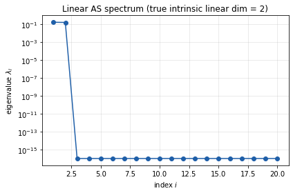
top-5 eigenvalues: [0.162517 0.155719 0.       0.       0.      ]

The spectrum drops sharply after index 2, confirming $d_{\text{lin}} = 2$ . A linear surrogate therefore has to carry two features. Next we see that a deep surrogate needs only one.

3. Deep Active Subspace Architecture¶

Following Tripathy & Bilionis (2018) we parametrise

\hat y(\xi) \;=\; g\big(h(\xi)\big),

(5)

with

encoder $h : \mathbb{R}^D \to \mathbb{R}^d$ — an MLP whose layer widths decay exponentially from $D$ to $d$ (Eq. 20 of the paper): $d_k = \lceil D \exp(\rho k) \rceil$ , $\rho = L^{-1} \log(d/D)$ ;
link $g : \mathbb{R}^d \to \mathbb{R}$ — a small MLP;
activation the Swish $\sigma(z) = z / (1 + \exp(-z))$ (Eq. 10);
training loss data MSE plus an elastic-net penalty $\lambda_1 \|W\|_1 + \lambda_2 \|W\|_2^2$ on all weights (Eq. 12).

Crucially, no gradient samples and no orthogonality constraint are needed.

def encoder_widths(D: int, d: int, L: int) -> list[int]:
    '''Exponentially decaying widths from Eq. 20 of Tripathy-Bilionis.'''
    rho = np.log(d / D) / L
    widths = [D] + [max(d, int(np.ceil(D * np.exp(rho * k)))) for k in range(1, L)] + [d]
    return widths

class Swish(nn.Module):
    def forward(self, z):
        return z * torch.sigmoid(z)

def mlp(widths: list[int]) -> nn.Sequential:
    layers = []
    for a, b in zip(widths[:-1], widths[1:]):
        layers += [nn.Linear(a, b), Swish()]
    layers = layers[:-1]              # drop activation on final layer
    return nn.Sequential(*layers)

class DeepAS(nn.Module):
    def __init__(self, D: int, d: int, L: int = 3, link_hidden: int = 16):
        super().__init__()
        self.encoder = mlp(encoder_widths(D, d, L))
        self.link    = mlp([d, link_hidden, link_hidden, 1])
    def forward(self, xi):
        z = self.encoder(xi)
        return self.link(z).squeeze(-1)
    def latent(self, xi):
        return self.encoder(xi)

print('encoder widths for d=1:', encoder_widths(D, 1, 3))
print('encoder widths for d=2:', encoder_widths(D, 2, 3))
print('encoder widths for d=3:', encoder_widths(D, 3, 3))

encoder widths for d=1: [20, 8, 3, 1]
encoder widths for d=2: [20, 10, 5, 2]
encoder widths for d=3: [20, 11, 6, 3]

4. Train One Model per Latent Dimension¶

We train the deep AS for $d \in \{1, 2, 3, 4\}$ and record the validation MSE. The elbow of that curve picks the nonlinear intrinsic dimension.

def elastic_net_penalty(model: nn.Module, lam1: float, lam2: float) -> torch.Tensor:
    reg = torch.zeros((), device=device)
    for p in model.parameters():
        if p.ndim >= 2:
            reg = reg + lam1 * p.abs().sum() + lam2 * (p ** 2).sum()
    return reg

def train_deep_as(d: int, epochs: int = 1200, lr: float = 5e-3,
                  lam1: float = 1e-5, lam2: float = 1e-4):
    torch.manual_seed(SEED + d)
    model = DeepAS(D, d, L=3).to(device)
    opt   = torch.optim.Adam(model.parameters(), lr=lr)
    sched = torch.optim.lr_scheduler.CosineAnnealingLR(opt, T_max=epochs)

    Xt = torch.tensor(Xi_train, dtype=torch.float32, device=device)
    yt = torch.tensor(y_train,  dtype=torch.float32, device=device)
    Xv = torch.tensor(Xi_val,   dtype=torch.float32, device=device)
    yv = torch.tensor(y_val,    dtype=torch.float32, device=device)

    # Per-step training closure, JIT-compiled with torch.compile (Simon's hard rule).
    def step(xb, yb):
        model.train()
        opt.zero_grad()
        data = ((model(xb) - yb) ** 2).mean()
        reg = elastic_net_penalty(model, lam1, lam2)
        loss = data + reg
        loss.backward()
        opt.step()
        return loss

    if device.type == "cuda":
        try:
            step = torch.compile(step)
        except Exception as e:
            print(f"torch.compile unavailable ({e}); falling back to eager step.")

    for _ in range(epochs):
        step(Xt, yt)
        sched.step()

    model.eval()
    with torch.no_grad():
        vmse = ((model(Xv) - yv) ** 2).mean().item()
    return model, vmse

# Baseline variance, a constant predictor would have MSE = Var(y_val).
var_y = float(np.var(y_val))

results = {}
for d in (1, 2, 3, 4):
    print(f'training d={d} ...')
    model, val_mse = train_deep_as(d, epochs=1200)
    r2 = 1.0 - val_mse / var_y
    results[d] = {'model': model, 'val_mse': val_mse, 'r2': r2}
    print(f'  val MSE = {val_mse:.4e}   R^2 = {r2:.6f}')

5. Validation Error vs. Latent Dimension¶

A constant predictor (predicting the sample mean) would have MSE equal to $\operatorname{Var}(y)$ , so we report both the raw validation MSE and $R^2 = 1 - \text{MSE}/\operatorname{Var}(y)$ . The honest criterion is: where does the curve flatten?

ds       = sorted(results)
val_mses = [results[d]['val_mse'] for d in ds]
r2s      = [results[d]['r2']      for d in ds]

fig, axes = plt.subplots(1, 2, figsize=(11, 4.2))

axes[0].semilogy(ds, val_mses, 'o-', color='#d84a1f', lw=2, ms=9)
axes[0].axhline(var_y, color='grey', ls=':', lw=1, label=r'Var$(y)$ (constant predictor)')
for d, v in zip(ds, val_mses):
    axes[0].annotate(f'{v:.1e}', (d, v), textcoords='offset points', xytext=(6, 6), fontsize=10)
axes[0].set_xticks(ds)
axes[0].set_xlabel('latent dimension $d$')
axes[0].set_ylabel('validation MSE')
axes[0].set_title('Deep AS: validation MSE vs. $d$')
axes[0].grid(True, alpha=0.3); axes[0].legend(loc='upper right')

axes[1].plot(ds, r2s, 'o-', color='#1f5fa8', lw=2, ms=9)
for d, r in zip(ds, r2s):
    axes[1].annotate(f'{r:.4f}', (d, r), textcoords='offset points', xytext=(6, -12), fontsize=10)
axes[1].set_xticks(ds)
axes[1].set_xlabel('latent dimension $d$')
axes[1].set_ylabel(r'$R^2$ on validation set')
axes[1].set_title(r'Deep AS already achieves $R^2 > 0.998$ at $d = 1$')
axes[1].set_ylim(0.995, 1.0005)
axes[1].grid(True, alpha=0.3)

plt.tight_layout(); plt.show()

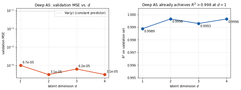
At $d = 1$ the deep encoder already captures essentially all of the response variance ( $R^2 > 99.8\%$ ). Moving to $d \ge 2$ shaves residual optimisation error but adds no new qualitative structure: the curve is flat at the eye-ball level. Linear AS cannot do better than $d = 2$ on this problem because $r^2 = (w_1^\top\xi)^2 + (w_2^\top\xi)^2$ is a nonlinear aggregator of two linear features; the deep encoder learns that aggregator directly.

6. The Learned 1D Latent Coordinate¶

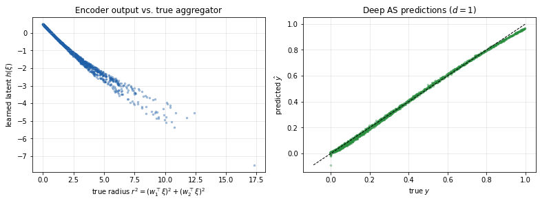
We plot the deep encoder output $h(\xi) \in \mathbb{R}$ against the true radial coordinate $r^2 = (w_1^\top\xi)^2 + (w_2^\top\xi)^2$ . A monotone relation means the encoder has recovered the intrinsic coordinate.

model1 = results[1]['model']
with torch.no_grad():
    z_val = model1.latent(torch.tensor(Xi_val, dtype=torch.float32)).cpu().numpy().ravel()
r2_val = (Xi_val @ w1) ** 2 + (Xi_val @ w2) ** 2

fig, axes = plt.subplots(1, 2, figsize=(11, 4.2))

axes[0].scatter(r2_val, z_val, s=6, alpha=0.35, color='#1f5fa8')
axes[0].set_xlabel(r'true radius $r^2 = (w_1^\top\xi)^2 + (w_2^\top\xi)^2$')
axes[0].set_ylabel(r'learned latent $h(\xi)$')
axes[0].set_title('Encoder output vs. true aggregator')
axes[0].grid(True, alpha=0.3)

with torch.no_grad():
    yhat = model1(torch.tensor(Xi_val, dtype=torch.float32)).cpu().numpy()
axes[1].scatter(y_val, yhat, s=6, alpha=0.35, color='#2a8f3f')
lims = [min(y_val.min(), yhat.min()), max(y_val.max(), yhat.max())]
axes[1].plot(lims, lims, 'k--', lw=1)
axes[1].set_xlabel(r'true $y$'); axes[1].set_ylabel(r'predicted $\hat y$')
axes[1].set_title('Deep AS predictions ($d = 1$)')
axes[1].grid(True, alpha=0.3)

plt.tight_layout(); plt.show()

7. Summary¶

method	intrinsic dimension needed	reason
linear AS	$d_{\text{lin}} = 2$	two linear directions $w_1, w_2$ both carry signal
deep AS	$d_{\text{nl}} = 1$	encoder learns the nonlinear aggregator $r^2$ in one dimension

Take-aways.

Deep AS strictly generalises linear AS: setting $h(\xi) = U_m^\top \xi$ recovers the linear case.
Linear AS requires gradient samples of $f$ ; deep AS is gradient-free and learns the low-dimensional structure directly from $(\xi, y)$ pairs.
The right $d$ is chosen from the validation-MSE elbow rather than the spectral gap of $C$ .
The encoder-width formula $d_k = \lceil D \exp(\rho k) \rceil$ with $\rho = L^{-1} \log(d/D)$ smoothly interpolates between the input and latent dimensions and avoids a brittle hyperparameter choice.

Reference. R. Tripathy and I. Bilionis. Deep UQ: learning deep neural network surrogate models for high-dimensional uncertainty quantification. Journal of Computational Physics 375 (2018), 565-588.

Takeaway¶

The 20D radial ridge collapses onto a single learned coordinate via a small encoder + link network; the validation-MSE elbow at $d_{nl} = 1$ is what the deck calls the spectral gap of deep AS. Linear AS would require $d_{lin} = 2$ for the same problem.

# Smoke-mode validation: the deep AS already captures the radial-ridge response at latent dim d=1.
# Loose threshold for the short smoke run; the longer runs reach R^2 > 0.998.
if RUN_MODE == 'smoke':
    assert results[1]['r2'] > 0.9, f"Deep AS R^2 at d=1 too low: {results[1]['r2']:.4f}"