Lecture 14, Notebook 08: Deep kernel learning — a neural feature extractor with a GP head - Deep Learning for Solving and Estimating Dynamic Models in Economics and Finance

Course: Deep Learning for Solving and Estimating Dynamic Models in Economics and Finance
Script reference: §9.7 (Deep kernel learning — neural feature extractor + GP head on a hidden-regime problem)
Notebook role: core
Author: Simon Scheidegger

RUN_MODE = "smoke"  # one of: "smoke", "teaching", "production"
SEED = 0

Overview¶

This notebook introduces deep kernels step by step.

The organizing idea is simple:

A plain Gaussian process (GP) assumes that distance in the raw input space is already meaningful.
A deep kernel first learns a feature map $\phi_\theta(x)$ with a neural network.
A GP is then applied to the learned representation instead of to the raw input:
$k_{\text{DKL}}(x, x') \;=\; k_{\text{base}}\!\left(\phi_\theta(x),\,\phi_\theta(x')\right).$
(1)

This notebook is intentionally pedagogical:

We begin with a warm-up where a standard GP is already enough.
We then construct a hidden-regime regression problem where raw stationary kernels struggle.
We show how a feature map that repairs the geometry helps the GP.
Finally, we train a small neural network to learn that feature map and benchmark the resulting learned-feature GP against standard RBF and Matern GPs.

Important teaching note¶

To keep the notebook transparent and fast, the feature-learning section uses a supervised proxy target for the latent coordinate. In production DKL, one would typically learn the feature extractor and GP jointly via the GP marginal likelihood (for example with GPyTorch). The present notebook focuses on the core geometry and benchmarking intuition.

Implementation note. This notebook implements DKL via a supervised feature extractor + sklearn GP head, not joint marginal-likelihood training with GPyTorch. The conceptual workflow is identical; the joint-likelihood version is left as an extension.

import numpy as np
import pandas as pd
import matplotlib.pyplot as plt
from sklearn.gaussian_process import GaussianProcessRegressor
from sklearn.gaussian_process.kernels import RBF, Matern, ConstantKernel as ConstantKernel
from sklearn.metrics import mean_squared_error
from sklearn.preprocessing import StandardScaler

import torch
import torch.nn as nn

SEED = 0
NOISE_STD = 0.05

np.random.seed(SEED)
rng = np.random.default_rng(SEED)
torch.manual_seed(SEED)

plt.rcParams['figure.figsize'] = (9, 5)
plt.rcParams['font.size'] = 13
plt.rcParams['axes.grid'] = True
plt.rcParams['grid.alpha'] = 0.25

def rmse(y_true, y_pred):
    return float(np.sqrt(mean_squared_error(y_true, y_pred)))

def gaussian_nlpd(y_true, mean, std):
    var = np.maximum(std**2, 1e-8)
    return float(0.5 * np.mean(np.log(2 * np.pi * var) + (y_true - mean) ** 2 / var))

def coverage_95(y_true, mean, std):
    return float(np.mean((y_true >= mean - 1.96 * std) & (y_true <= mean + 1.96 * std)))

def observation_std(latent_std, noise_std=NOISE_STD):
    # sklearn returns latent-function uncertainty; for predictive intervals we add observation noise back in.
    return np.sqrt(latent_std**2 + noise_std**2)

print('Imports successful.')
print(f'PyTorch version: {torch.__version__}')

# Hyperparameter budget, dispatched on RUN_MODE (see the run-mode cell above).
if RUN_MODE == "smoke":
    DKL_EPOCHS, DKL_BATCH = 200, 64
elif RUN_MODE == "teaching":
    DKL_EPOCHS, DKL_BATCH = 800, 128
elif RUN_MODE == "production":
    DKL_EPOCHS, DKL_BATCH = 3_000, 256
else:
    raise ValueError(f"Unknown RUN_MODE={RUN_MODE!r}")

1. Warm-up: When a Plain GP Is Already Enough¶

Before adding neural feature maps, it is useful to see the case where a standard GP is already the right tool.

We generate a smooth one-dimensional function,

f(x) = \sin(x) + 0.2x,

(2)

and fit a standard RBF GP.

This is exactly the kind of problem where a plain GP shines:

the input is already low-dimensional,
the geometry is simple,
the target is smooth,
and uncertainty quantification comes for free.


X_train_1d = np.linspace(-4.0, 4.0, 18).reshape(-1, 1)
y_train_1d = np.sin(X_train_1d[:, 0]) + 0.2 * X_train_1d[:, 0] + rng.normal(scale=0.05, size=len(X_train_1d))

X_test_1d = np.linspace(-4.5, 4.5, 300).reshape(-1, 1)
y_true_1d = np.sin(X_test_1d[:, 0]) + 0.2 * X_test_1d[:, 0]

rbf_1d = GaussianProcessRegressor(
    kernel=ConstantKernel(1.0, (1e-2, 1e2)) * RBF(length_scale=1.0, length_scale_bounds=(1e-2, 1e2)),
    alpha=1e-4,
    normalize_y=True,
    n_restarts_optimizer=3,
    random_state=SEED,
)
rbf_1d.fit(X_train_1d, y_train_1d)
mean_1d, std_1d = rbf_1d.predict(X_test_1d, return_std=True)

fig, ax = plt.subplots(figsize=(10, 4.5))
ax.plot(X_test_1d[:, 0], y_true_1d, color='black', linestyle='--', linewidth=1.5, label='True function')
ax.plot(X_test_1d[:, 0], mean_1d, color='tab:blue', linewidth=2.0, label='RBF GP mean')
ax.fill_between(
    X_test_1d[:, 0],
    mean_1d - 1.96 * std_1d,
    mean_1d + 1.96 * std_1d,
    color='tab:blue',
    alpha=0.2,
    label='95% interval',
)
ax.scatter(X_train_1d[:, 0], y_train_1d, color='tab:red', s=35, zorder=5, label='Training data')
ax.set_title('Warm-up: standard RBF GP on a smooth 1D problem')
ax.set_xlabel('x')
ax.set_ylabel('y')
ax.legend(loc='upper left')
plt.tight_layout()
plt.show()

print(f'Warm-up RMSE: {rmse(y_true_1d, mean_1d):.4f}')

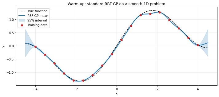
Warm-up RMSE: 0.0505

The warm-up already suggests the right philosophy:

Do not use deep kernels by default.
Use them when the raw input geometry is the bottleneck, not when a plain GP already works.

We now build a synthetic example where the raw geometry is the bottleneck.

2. A Hidden-Regime Problem Where Raw Stationary Kernels Struggle¶

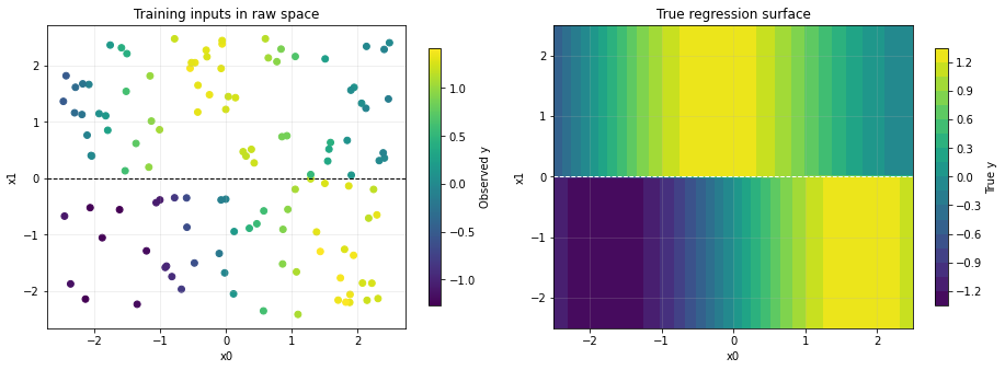
We now create a two-dimensional dataset with a hidden phase shift.

Let

u(x_0, x_1) = x_0 + 2 \cdot \mathbf{1}\{x_1 \ge 0\},

(3)

and define the regression target as

y = \sin(u) + 0.2\,u + \varepsilon.

(4)

Why this is interesting¶

In the latent coordinate $u$ , the function is smooth and easy.
In the raw coordinates $(x_0, x_1)$ , crossing the boundary $x_1 = 0$ causes a regime-dependent phase shift.
A stationary raw-input kernel such as RBF or Matern tends to blur information across that boundary.

This is the exact situation where a deep kernel can help: the neural network learns a representation in which the GP sees a smoother problem.

N_TRAIN = 120
N_TEST = 400

X_train = rng.uniform(-2.5, 2.5, size=(N_TRAIN, 2))
X_test = rng.uniform(-2.5, 2.5, size=(N_TEST, 2))

def latent_u(X):
    x0 = X[:, 0]
    x1 = X[:, 1]
    return x0 + 2.0 * (x1 >= 0.0)

def target_function(X):
    u = latent_u(X)
    return np.sin(u) + 0.2 * u

def teacher_feature(X):
    return (X[:, 0] + 2.0 / (1.0 + np.exp(-8.0 * X[:, 1]))).reshape(-1, 1)

# The observed targets are noisy, while the test targets below stay noise-free so we can judge mean prediction cleanly.
y_train = target_function(X_train) + rng.normal(scale=NOISE_STD, size=N_TRAIN)
y_test = target_function(X_test)

x0_grid = np.linspace(-2.5, 2.5, 120)
x1_grid = np.linspace(-2.5, 2.5, 120)
X0, X1 = np.meshgrid(x0_grid, x1_grid)
X_grid = np.column_stack([X0.ravel(), X1.ravel()])
y_true_grid = target_function(X_grid).reshape(X0.shape)

print('Training set shape:', X_train.shape)
print('Test set shape:', X_test.shape)
print(f'Target range: [{y_train.min():.3f}, {y_train.max():.3f}]')

Training set shape: (120, 2)
Test set shape: (400, 2)
Target range: [-1.271, 1.422]


fig, axes = plt.subplots(1, 2, figsize=(13, 4.8))

sc = axes[0].scatter(X_train[:, 0], X_train[:, 1], c=y_train, cmap='viridis', s=35)
axes[0].axhline(0.0, color='black', linestyle='--', linewidth=1.0)
axes[0].set_title('Training inputs in raw space')
axes[0].set_xlabel('x0')
axes[0].set_ylabel('x1')
plt.colorbar(sc, ax=axes[0], shrink=0.85, label='Observed y')

cont = axes[1].contourf(X0, X1, y_true_grid, levels=25, cmap='viridis')
axes[1].axhline(0.0, color='white', linestyle='--', linewidth=1.0)
axes[1].set_title('True regression surface')
axes[1].set_xlabel('x0')
axes[1].set_ylabel('x1')
plt.colorbar(cont, ax=axes[1], shrink=0.85, label='True y')

plt.tight_layout()
plt.show()

3. Raw-Input GP Baselines¶

We now fit two standard GP regressors directly on the raw input pair $(x_0, x_1)$ :

RBF GP (squared exponential / Gaussian kernel)
Matern GP with $u = 3/2$

Both models are given the same standardized inputs and allowed to learn their hyperparameters via marginal likelihood.

x_scaler = StandardScaler().fit(X_train)
X_train_std = x_scaler.transform(X_train)
X_test_std = x_scaler.transform(X_test)
X_grid_std = x_scaler.transform(X_grid)

raw_models = {
    'RBF GP': GaussianProcessRegressor(
        kernel=ConstantKernel(1.0, (1e-2, 1e2)) * RBF(length_scale=np.ones(2), length_scale_bounds=(1e-2, 1e2)),
        alpha=1e-4,
        normalize_y=True,
        n_restarts_optimizer=3,
        random_state=SEED,
    ),
    'Matern GP': GaussianProcessRegressor(
        kernel=ConstantKernel(1.0, (1e-2, 1e2)) * Matern(length_scale=np.ones(2), length_scale_bounds=(1e-2, 1e2), nu=1.5),
        alpha=1e-4,
        normalize_y=True,
        n_restarts_optimizer=3,
        random_state=SEED,
    ),
}

results = []
model_store = {}

for name, model in raw_models.items():
    model.fit(X_train_std, y_train)
    mean_test, std_test = model.predict(X_test_std, return_std=True)
    mean_grid, std_grid = model.predict(X_grid_std, return_std=True)
    obs_std_test = observation_std(std_test)

    results.append({
        'Model': name,
        'RMSE': rmse(y_test, mean_test),
        'ObsNLPD': gaussian_nlpd(y_test, mean_test, obs_std_test),
        'ObsCoverage95': coverage_95(y_test, mean_test, obs_std_test),
    })
    model_store[name] = {
        'model': model,
        'mean_test': mean_test,
        'std_test': std_test,
        'obs_std_test': obs_std_test,
        'mean_grid': mean_grid.reshape(X0.shape),
        'std_grid': std_grid.reshape(X0.shape),
    }
    print(name)
    print('  learned kernel:', model.kernel_)
    print(f"  RMSE        = {results[-1]['RMSE']:.4f}")
    print(f"  Obs. NLPD   = {results[-1]['ObsNLPD']:.4f}")
    print(f"  Obs. 95% cov= {results[-1]['ObsCoverage95']:.3f}")

RBF GP
  learned kernel: 0.907**2 * RBF(length_scale=[0.545, 0.121])
  RMSE        = 0.3720
  Obs. NLPD   = 0.1840
  Obs. 95% cov= 0.880

Matern GP
  learned kernel: 1.09**2 * Matern(length_scale=[1.46, 0.392], nu=1.5)
  RMSE        = 0.1414
  Obs. NLPD   = -0.6784
  Obs. 95% cov= 0.968


fig, axes = plt.subplots(1, 3, figsize=(16, 4.8), sharex=True, sharey=True)

panels = [
    ('Truth', y_true_grid),
    ('RBF GP', model_store['RBF GP']['mean_grid']),
    ('Matern GP', model_store['Matern GP']['mean_grid']),
]

for ax, (title, surface) in zip(axes, panels):
    contour = ax.contourf(X0, X1, surface, levels=25, cmap='viridis')
    ax.scatter(X_train[:, 0], X_train[:, 1], c='white', s=10, alpha=0.7)
    ax.axhline(0.0, color='black', linestyle='--', linewidth=1.0)
    ax.set_title(title)
    ax.set_xlabel('x0')
    ax.set_ylabel('x1')
    plt.colorbar(contour, ax=ax, shrink=0.85)

plt.suptitle('Raw-input GP surfaces', y=1.02)
plt.tight_layout()
plt.show()

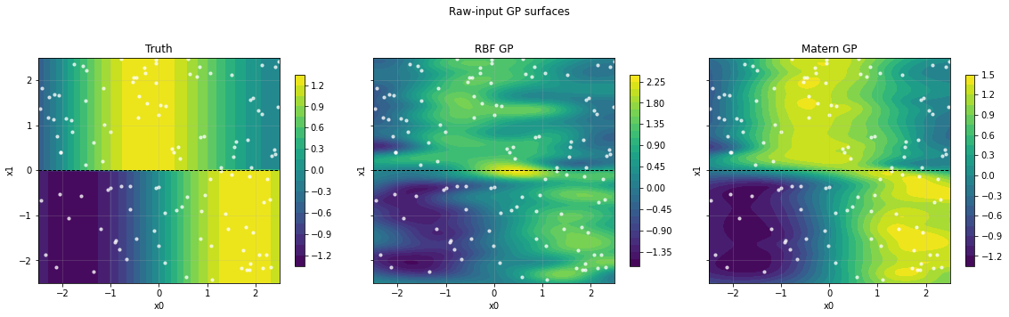
Even before introducing the deep kernel, the failure mode is visible:

both raw-input GPs are trying to use a single stationary metric in $(x_0, x_1)$ ,
so they blur across the hidden boundary,
and the phase shift is not represented as cleanly as it should be.

The next step is to change the geometry seen by the GP.

4. A Teacher Deep Kernel¶

To make the geometry explicit, define the smooth feature map

\phi_{\text{teacher}}(x_0, x_1) \;=\; x_0 + 2\,\sigma(8 x_1),

(5)

where $\sigma(z) = \dfrac{1}{1 + e^{-z}}$ is the logistic sigmoid.

This feature map does exactly what we want:

when $x_1 < 0$ , it leaves the coordinate close to $x_0$ ,
when $x_1 > 0$ , it shifts the coordinate by roughly +2,
so the latent smooth target becomes much easier for a 1D GP.

We now fit a GP on $\phi_{\text{teacher}}(x)$ instead of on the raw pair $(x_0, x_1)$ .

teacher_train = teacher_feature(X_train)
teacher_test = teacher_feature(X_test)
teacher_grid = teacher_feature(X_grid)

teacher_scaler = StandardScaler().fit(teacher_train)
teacher_train_std = teacher_scaler.transform(teacher_train)
teacher_test_std = teacher_scaler.transform(teacher_test)
teacher_grid_std = teacher_scaler.transform(teacher_grid)

teacher_gp = GaussianProcessRegressor(
    kernel=ConstantKernel(1.0, (1e-2, 1e2)) * RBF(length_scale=1.0, length_scale_bounds=(1e-2, 1e2)),
    alpha=0.01,
    normalize_y=True,
    n_restarts_optimizer=5,
    random_state=SEED,
)
teacher_gp.fit(teacher_train_std, y_train)
teacher_mean_test, teacher_std_test = teacher_gp.predict(teacher_test_std, return_std=True)
teacher_mean_grid, teacher_std_grid = teacher_gp.predict(teacher_grid_std, return_std=True)
teacher_obs_std_test = observation_std(teacher_std_test)

results.append({
    'Model': 'Teacher deep-kernel GP',
    'RMSE': rmse(y_test, teacher_mean_test),
    'ObsNLPD': gaussian_nlpd(y_test, teacher_mean_test, teacher_obs_std_test),
    'ObsCoverage95': coverage_95(y_test, teacher_mean_test, teacher_obs_std_test),
})
model_store['Teacher deep-kernel GP'] = {
    'model': teacher_gp,
    'mean_test': teacher_mean_test,
    'std_test': teacher_std_test,
    'obs_std_test': teacher_obs_std_test,
    'mean_grid': teacher_mean_grid.reshape(X0.shape),
    'std_grid': teacher_std_grid.reshape(X0.shape),
}

print('Teacher deep-kernel GP')
print('  learned top kernel:', teacher_gp.kernel_)
print(f"  RMSE        = {results[-1]['RMSE']:.4f}")
print(f"  Obs. NLPD   = {results[-1]['ObsNLPD']:.4f}")
print(f"  Obs. 95% cov= {results[-1]['ObsCoverage95']:.3f}")

Teacher deep-kernel GP
  learned top kernel: 1.36**2 * RBF(length_scale=1.2)
  RMSE        = 0.1180
  Obs. NLPD   = 0.4891
  Obs. 95% cov= 0.902


fig, axes = plt.subplots(1, 2, figsize=(13, 4.5))

axes[0].scatter(X_train[:, 0], X_train[:, 1], c=teacher_train[:, 0], cmap='coolwarm', s=35)
axes[0].axhline(0.0, color='black', linestyle='--', linewidth=1.0)
axes[0].set_title('Teacher feature value in raw space')
axes[0].set_xlabel('x0')
axes[0].set_ylabel('x1')

contour = axes[1].contourf(X0, X1, model_store['Teacher deep-kernel GP']['mean_grid'], levels=25, cmap='viridis')
axes[1].scatter(X_train[:, 0], X_train[:, 1], c='white', s=10, alpha=0.7)
axes[1].axhline(0.0, color='black', linestyle='--', linewidth=1.0)
axes[1].set_title('Teacher deep-kernel GP surface')
axes[1].set_xlabel('x0')
axes[1].set_ylabel('x1')
plt.colorbar(contour, ax=axes[1], shrink=0.85)

plt.tight_layout()
plt.show()

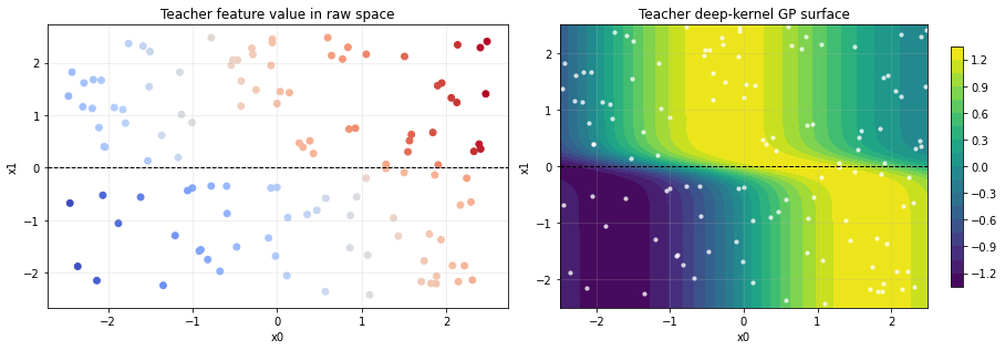
This is the deep-kernel idea in its cleanest form:

the GP itself is still just a GP,
the gain comes from changing the input representation,
and once the representation is good, even a simple 1D RBF kernel performs very well.

Next we replace the teacher feature map by a learned neural approximation.

5. Learn the Feature Map with a Small Neural Network¶

To keep the notebook fully transparent, we train a small neural network to approximate the teacher feature

\phi_{\text{teacher}}(x).

(6)

This is a pedagogical proxy for deep kernel learning:

the network learns a task-relevant representation,
the GP is placed on that representation,
and the benchmark can then be compared directly to raw RBF and Matern GPs.

We still report GP-based observation intervals, but there is an important caveat:

because the feature extractor is trained in a separate first stage here,
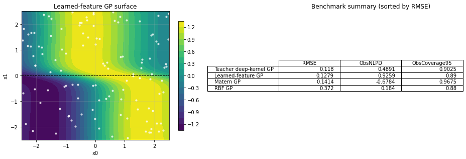
uncertainty calibration is not as strong as in a fully joint DKL fit,
so the cleanest performance comparison in this notebook is the mean-prediction gain and the regime-recovery plots.

In a production DKL setup, one would replace this supervised feature-matching step with joint optimization of feature extractor + GP marginal likelihood.

class FeatureNet(nn.Module):
    # Small neural net mapping raw 2D inputs to a 1D latent feature.
    def __init__(self):
        super().__init__()
        self.net = nn.Sequential(
            nn.Linear(2, 32),
            nn.Tanh(),
            nn.Linear(32, 16),
            nn.Tanh(),
            nn.Linear(16, 1),
        )

    def forward(self, x):
        return self.net(x)

feature_net = FeatureNet()
optimizer = torch.optim.Adam(feature_net.parameters(), lr=0.01, weight_decay=1e-4)

X_train_t = torch.tensor(X_train_std, dtype=torch.float32)
teacher_train_t = torch.tensor(teacher_train_std, dtype=torch.float32)


# Per-batch training step, JIT-compiled with torch.compile (Simon's hard rule).
def feature_step(x, target):
    pred = feature_net(x)
    loss = torch.mean((pred - target) ** 2)
    optimizer.zero_grad()
    loss.backward()
    optimizer.step()
    return loss

try:
    feature_step = torch.compile(feature_step)
except Exception as e:
    print(f"torch.compile unavailable ({e}); falling back to eager step.")

loss_history = []
for epoch in range(500):
    loss = feature_step(X_train_t, teacher_train_t)
    loss_history.append(float(loss.item()))

with torch.no_grad():
    learned_train = feature_net(torch.tensor(X_train_std, dtype=torch.float32)).numpy()
    learned_test = feature_net(torch.tensor(X_test_std, dtype=torch.float32)).numpy()
    learned_grid = feature_net(torch.tensor(X_grid_std, dtype=torch.float32)).numpy()

print(f'Final feature-learning loss: {loss_history[-1]:.6f}')


fig, axes = plt.subplots(1, 2, figsize=(12, 4.3))

axes[0].plot(loss_history, color='tab:blue')
axes[0].set_title('Feature-learning loss')
axes[0].set_xlabel('Epoch')
axes[0].set_ylabel('MSE')

axes[1].scatter(teacher_test_std[:, 0], learned_test[:, 0], s=18, alpha=0.75, color='tab:purple')
line_min = min(teacher_test_std[:, 0].min(), learned_test[:, 0].min())
line_max = max(teacher_test_std[:, 0].max(), learned_test[:, 0].max())
axes[1].plot([line_min, line_max], [line_min, line_max], color='black', linestyle='--')
axes[1].set_title('Learned feature vs teacher feature')
axes[1].set_xlabel('Teacher feature (standardized)')
axes[1].set_ylabel('Learned feature')

plt.tight_layout()
plt.show()

print(f'Feature RMSE on the test set: {rmse(teacher_test_std[:, 0], learned_test[:, 0]):.4f}')

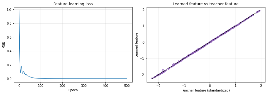
Feature RMSE on the test set: 0.0145

learned_gp = GaussianProcessRegressor(
    kernel=ConstantKernel(1.0, (1e-2, 1e2)) * RBF(length_scale=1.0, length_scale_bounds=(1e-2, 1e2)),
    alpha=0.01,
    normalize_y=True,
    n_restarts_optimizer=5,
    random_state=SEED,
)
learned_gp.fit(learned_train, y_train)
learned_mean_test, learned_std_test = learned_gp.predict(learned_test, return_std=True)
learned_mean_grid, learned_std_grid = learned_gp.predict(learned_grid, return_std=True)
learned_obs_std_test = observation_std(learned_std_test)

results.append({
    'Model': 'Learned-feature GP',
    'RMSE': rmse(y_test, learned_mean_test),
    'ObsNLPD': gaussian_nlpd(y_test, learned_mean_test, learned_obs_std_test),
    'ObsCoverage95': coverage_95(y_test, learned_mean_test, learned_obs_std_test),
})
model_store['Learned-feature GP'] = {
    'model': learned_gp,
    'mean_test': learned_mean_test,
    'std_test': learned_std_test,
    'obs_std_test': learned_obs_std_test,
    'mean_grid': learned_mean_grid.reshape(X0.shape),
    'std_grid': learned_std_grid.reshape(X0.shape),
}

print('Learned-feature GP')
print('  learned top kernel:', learned_gp.kernel_)
print(f"  RMSE        = {results[-1]['RMSE']:.4f}")
print(f"  Obs. NLPD   = {results[-1]['ObsNLPD']:.4f}")
print(f"  Obs. 95% cov= {results[-1]['ObsCoverage95']:.3f}")

Learned-feature GP
  learned top kernel: 1.37**2 * RBF(length_scale=1.21)
  RMSE        = 0.1279
  Obs. NLPD   = 0.9259
  Obs. 95% cov= 0.890

fig, axes = plt.subplots(1, 2, figsize=(13, 4.5))

contour = axes[0].contourf(X0, X1, model_store['Learned-feature GP']['mean_grid'], levels=25, cmap='viridis')
axes[0].scatter(X_train[:, 0], X_train[:, 1], c='white', s=10, alpha=0.7)
axes[0].axhline(0.0, color='black', linestyle='--', linewidth=1.0)
axes[0].set_title('Learned-feature GP surface')
axes[0].set_xlabel('x0')
axes[0].set_ylabel('x1')
plt.colorbar(contour, ax=axes[0], shrink=0.85)

comparison = pd.DataFrame(results).set_index('Model').sort_values('RMSE').round(4)
axes[1].axis('off')
axes[1].table(
    cellText=comparison.values,
    rowLabels=comparison.index,
    colLabels=comparison.columns,
    loc='center',
)
axes[1].set_title('Benchmark summary (sorted by RMSE)')

plt.tight_layout()
plt.show()

comparison

6. Slice Plots: Where the Deep Kernel Helps¶

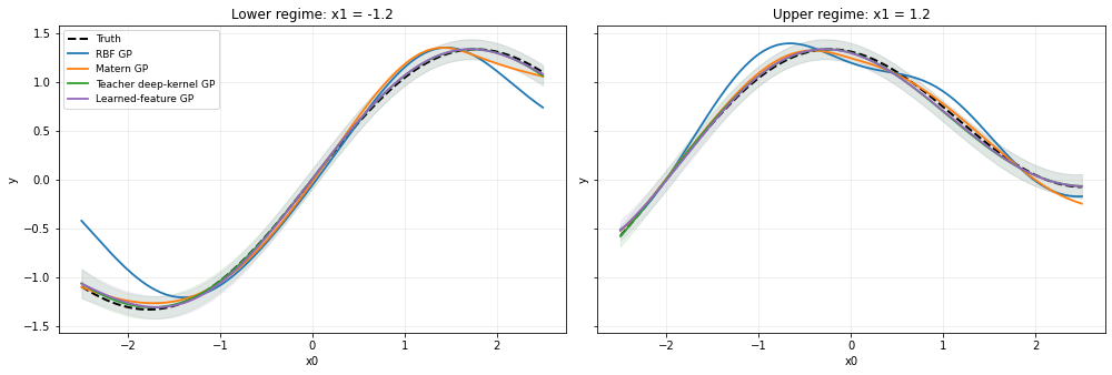
A good way to see the problem is to hold $x_1$ fixed and sweep over $x_0$ .

We look at two slices:

one in the lower regime ( $x_1 < 0$ ),
one in the upper regime ( $x_1 > 0$ ).

A stationary raw-input GP tries to compromise across both regimes, while the deep-kernel feature map explicitly aligns them.

def predict_raw(model, X_raw):
    X_std = x_scaler.transform(X_raw)
    mean, std = model.predict(X_std, return_std=True)
    return mean, observation_std(std)

def predict_teacher(X_raw):
    feat = teacher_scaler.transform(teacher_feature(X_raw))
    mean, std = teacher_gp.predict(feat, return_std=True)
    return mean, observation_std(std)

def predict_learned(X_raw):
    feat = feature_net(torch.tensor(x_scaler.transform(X_raw), dtype=torch.float32)).detach().numpy()
    mean, std = learned_gp.predict(feat, return_std=True)
    return mean, observation_std(std)

x0_line = np.linspace(-2.5, 2.5, 300)
regimes = [(-1.2, 'Lower regime: x1 = -1.2'), (1.2, 'Upper regime: x1 = 1.2')]
colors = {
    'Truth': 'black',
    'RBF GP': 'tab:blue',
    'Matern GP': 'tab:orange',
    'Teacher deep-kernel GP': 'tab:green',
    'Learned-feature GP': 'tab:purple',
}

fig, axes = plt.subplots(1, 2, figsize=(14, 4.8), sharey=True)
for ax, (x1_fixed, title) in zip(axes, regimes):
    X_line = np.column_stack([x0_line, np.full_like(x0_line, x1_fixed)])
    y_line_true = target_function(X_line)

    ax.plot(x0_line, y_line_true, color=colors['Truth'], linestyle='--', linewidth=2.0, label='Truth')

    for name in ['RBF GP', 'Matern GP']:
        mean, std = predict_raw(model_store[name]['model'], X_line)
        ax.plot(x0_line, mean, color=colors[name], linewidth=1.8, label=name)

    for name, predictor in [
        ('Teacher deep-kernel GP', predict_teacher),
        ('Learned-feature GP', predict_learned),
    ]:
        mean, std = predictor(X_line)
        ax.plot(x0_line, mean, color=colors[name], linewidth=1.8, label=name)
        ax.fill_between(x0_line, mean - 1.96 * std, mean + 1.96 * std, color=colors[name], alpha=0.10)

    ax.set_title(title)
    ax.set_xlabel('x0')
    ax.set_ylabel('y')

axes[0].legend(loc='upper left', fontsize=9)
plt.tight_layout()
plt.show()

7. What This Notebook Shows¶

Main lesson¶

A deep kernel helps when the target is smooth in a latent coordinate system, but not in the raw coordinates seen by a standard stationary GP.

In this notebook¶

The raw RBF GP is the weakest baseline because it uses a single stationary geometry in raw space.
The raw Matern GP is more robust, but still constrained by the same raw geometry.
The teacher deep-kernel GP gives the lowest RMSE and the cleanest recovery of the hidden regime structure.
The learned-feature GP recovers most of that gain once the feature map is learned.

How to read the benchmark table¶

RMSE is the clearest score for the representation-learning gain in this two-stage notebook.
ObsNLPD and ObsCoverage95 evaluate observation intervals after adding measurement noise back to the GP variance.
Because the feature map is learned in a separate proxy stage here, uncertainty calibration is still not as strong as in a fully end-to-end DKL model.

Practical interpretation¶

In real applied work, the unknown part is the feature map $\phi_\theta(x)$ . Deep kernel learning replaces the hand-crafted or teacher feature map with a neural network and trains it from data so that the GP sees a representation where a simple kernel is once again appropriate.

Takeaway¶

On the hidden-regime 2D problem, raw-input GPs blur across the regime boundary, the teacher deep kernel restores it, and the supervised proxy reaches most of that gain. For the joint marginal-likelihood form (true DKL) see GPyTorch\u2019s DeepKernel; the L14 deck flags the same caveat next to the DKL diagram.

# Smoke-mode validation: at least one GP variant achieves a reasonable RMSE on the benchmark.
if RUN_MODE == 'smoke':
    _best_rmse = float(comparison['RMSE'].iloc[0])
    assert _best_rmse < 1.0, f'Best benchmark RMSE too large: {_best_rmse:.3e}'