Course: Deep Learning for Solving and Estimating Dynamic Models in Economics and Finance
Script reference: §7.2 (the PINN loss and automatic differentiation; the 1D ODE example)
Notebook role: core
Author: Simon Scheidegger
Run mode. The checked-in run uses
RUN_MODE = "smoke"for fast execution; the accuracy figures quoted in the slides and the companion script use the longerteaching/productionbudgets. SetRUN_MODEin the next cell accordingly to reproduce them.
RUN_MODE = "smoke"  # one of: "smoke", "teaching", "production"
SEED = 0
Physics-Informed Neural Networks: 1D ODE with Zero Boundary Conditions¶
Physics-Informed Neural Networks (PINNs) embed the governing equations of a physical system directly into the loss function of a neural network. Instead of learning purely from data, the network is trained to satisfy:
The differential equation (the “physics”) at a set of collocation points in the domain.
The boundary conditions (and/or initial conditions) at the domain boundaries.
Because modern deep-learning frameworks provide automatic differentiation, we can compute exact derivatives of the network output with respect to its inputs and penalize any violation of the ODE/PDE.
Problem statement¶
We consider the simplest possible second-order ODE with homogeneous (zero) Dirichlet boundary conditions:
The analytical solution is
We will train a small fully connected neural network to approximate this solution using PyTorch.
Self-study notebook \u2014 This notebook complements the in-class PINNs session (Day 6, Block 1). Work through it at your own pace.
import torch
import torch.nn as nn
import torch.optim as optim
import numpy as np
import matplotlib.pyplot as plt

plt.rcParams['font.size'] = 13

# For reproducibility
torch.manual_seed(SEED)
np.random.seed(SEED)

# Use GPU if available
device = torch.device("cuda" if torch.cuda.is_available() else "cpu")
print(f"Using device: {device}")

# torch.compile is wrapped on per-batch steps below for JIT speedups.
# PINN-style losses use torch.autograd.grad with create_graph=True (double
# backward), which the default aot_autograd backend in PyTorch 2.x does not
# yet support. We use backend='eager' and allow dynamo to fall back to eager
# Python whenever it cannot trace a sub-call (e.g. clip_grad_norm_).
import torch._dynamo
torch._dynamo.config.suppress_errors = True
Using device: cpu
# Run-mode budget: hyperparameters dispatched from RUN_MODE (set in the second cell).
#   smoke      -- CPU-bounded smoke run for CI
#   teaching   -- laptop-scale figures
#   production -- full reproduction
_RUN_HP = {
    "smoke":      {"epochs":   500, "n_interior":  20, "lr": 1e-3, "print_every":  100},
    "teaching":   {"epochs":  5000, "n_interior":  50, "lr": 1e-3, "print_every":  500},
    "production": {"epochs": 20000, "n_interior": 200, "lr": 1e-3, "print_every": 2000},
}
if RUN_MODE not in _RUN_HP:
    raise ValueError(f"RUN_MODE must be one of {list(_RUN_HP)}")
HP = _RUN_HP[RUN_MODE]
print(f"RUN_MODE={RUN_MODE!r}; SEED={SEED}; hyperparameters: {HP}")
RUN_MODE='smoke'; SEED=0; hyperparameters: {'epochs': 500, 'n_interior': 20, 'lr': 0.001, 'print_every': 100}
Network Architecture¶
We use a simple multi-layer perceptron (MLP) with two hidden layers of 20 neurons
each. The activation function is Tanh, which is infinitely differentiable
(). This smoothness is important because PINNs require computing
higher-order derivatives of the network output with respect to its inputs via
automatic differentiation. Using a non-smooth activation such as ReLU would
produce zero (or undefined) second derivatives almost everywhere, making it
unsuitable for our second-order ODE.
class ODE_Net(nn.Module):
    """Simple MLP for approximating the ODE solution.

    Architecture: 1 -> 20 -> 20 -> 1 with Tanh activations.
    """

    def __init__(self):
        super().__init__()
        self.net = nn.Sequential(
            nn.Linear(1, 20),
            nn.Tanh(),
            nn.Linear(20, 20),
            nn.Tanh(),
            nn.Linear(20, 1),
        )

    def forward(self, x):
        return self.net(x)


model = ODE_Net().to(device)
print(model)
print(f"\nTotal trainable parameters: {sum(p.numel() for p in model.parameters())}")
ODE_Net(
(net): Sequential(
(0): Linear(in_features=1, out_features=20, bias=True)
(1): Tanh()
(2): Linear(in_features=20, out_features=20, bias=True)
(3): Tanh()
(4): Linear(in_features=20, out_features=1, bias=True)
)
)
Total trainable parameters: 481
Computing the PDE Residual via Automatic Differentiation¶
The key ingredient of a PINN is the residual of the differential equation, evaluated using the network’s current predictions. For our ODE the residual is
We compute the first and second derivatives with torch.autograd.grad. The flag
create_graph=True is essential: it tells PyTorch to build a computational graph
for the derivative itself, so that we can (a) differentiate again to get the second
derivative and (b) backpropagate through the residual during training.
def residual(model, x):
    """Compute the ODE residual r(x) = y''(x) + 1.

    Parameters
    ----------
    model : ODE_Net
        The neural network approximating y(x).
    x : torch.Tensor
        Collocation points (requires_grad must be True).

    Returns
    -------
    torch.Tensor
        The residual y''(x) + 1 at each collocation point.
    """
    y = model(x)

    # First derivative dy/dx
    dy_dx = torch.autograd.grad(
        y, x,
        grad_outputs=torch.ones_like(y),
        create_graph=True,
    )[0]

    # Second derivative d^2y/dx^2
    d2y_dx2 = torch.autograd.grad(
        dy_dx, x,
        grad_outputs=torch.ones_like(dy_dx),
        create_graph=True,
    )[0]

    return d2y_dx2 + 1.0
Training the PINN¶
The total loss is the sum of two terms:
PDE loss -- mean squared residual over a set of interior collocation points:
Boundary condition (BC) loss -- squared error at the two endpoints:
We minimize with the Adam optimizer.
# ----- Hyperparameters (dispatched from RUN_MODE) -----
n_interior  = HP["n_interior"]
epochs      = HP["epochs"]
lr          = HP["lr"]
print_every = HP["print_every"]

# ----- Optimizer -----
optimizer = optim.Adam(model.parameters(), lr=lr)

# ----- Boundary points (fixed) -----
x_bc0 = torch.zeros(1, 1, device=device)   # x = 0
x_bc1 = torch.ones(1, 1, device=device)    # x = 1


def train_step(x_interior):
    optimizer.zero_grad()
    res = residual(model, x_interior)
    loss_pde = torch.mean(res ** 2)
    loss_bc = model(x_bc0) ** 2 + model(x_bc1) ** 2
    loss = loss_pde + loss_bc
    loss.backward()
    optimizer.step()
    return loss, loss_pde, loss_bc


# torch.compile per-batch step (backend="eager", fullgraph=False:
# residual uses torch.autograd.grad with create_graph=True for second derivatives,
# which the default aot_autograd backend in PyTorch 2.x does not yet support.)
train_step = torch.compile(train_step, fullgraph=False, backend="eager")

# ----- Training loop -----
loss_history = []

for epoch in range(1, epochs + 1):
    x_interior = torch.rand(n_interior, 1, device=device, requires_grad=True)
    loss, loss_pde, loss_bc = train_step(x_interior)
    loss_history.append(loss.item())

    if epoch % print_every == 0 or epoch == 1:
        print(
            f"Epoch {epoch:5d}/{epochs} | "
            f"Loss {loss.item():.3e}  "
            f"(PDE: {loss_pde.item():.3e}, BC: {loss_bc.item():.3e})"
        )

print("\nTraining complete.")
W0512 15:31:24.427000 98477 torch/_logging/_internal.py:1130] [7/0] Profiler function <class 'torch.autograd.profiler.record_function'> will be ignored
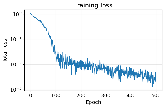
Epoch     1/500 | Loss 1.060e+00  (PDE: 9.497e-01, BC: 1.099e-01)
Epoch   100/500 | Loss 3.038e-02  (PDE: 2.962e-02, BC: 7.613e-04)
Epoch   200/500 | Loss 1.438e-02  (PDE: 1.434e-02, BC: 3.894e-05)
Epoch   300/500 | Loss 6.477e-03  (PDE: 6.473e-03, BC: 4.285e-06)
Epoch   400/500 | Loss 2.863e-03  (PDE: 2.838e-03, BC: 2.511e-05)
Epoch   500/500 | Loss 3.002e-03  (PDE: 2.990e-03, BC: 1.223e-05)

Training complete.
Evaluation and Visualization¶
We compare the trained network’s prediction with the analytical solution on a fine grid and visualize both the solution and the absolute pointwise error.
# ----- Evaluation grid -----
x_eval = torch.linspace(0, 1, 100, device=device).reshape(-1, 1)

with torch.no_grad():
    y_pred = model(x_eval).cpu().numpy()

x_np = x_eval.cpu().numpy()
y_exact = x_np * (1.0 - x_np) / 2.0    # analytical solution

# ----- Plot: PINN vs Analytical -----
fig, axes = plt.subplots(1, 2, figsize=(12, 4))

# Left panel: solutions
axes[0].plot(x_np, y_exact, "k-", linewidth=2, label="Analytical")
axes[0].plot(x_np, y_pred, "r--", linewidth=2, label="PINN")
axes[0].set_xlabel("x")
axes[0].set_ylabel("y(x)")
axes[0].set_title("Solution comparison")
axes[0].legend()
axes[0].grid(True, alpha=0.3)

# Right panel: absolute error
abs_error = np.abs(y_pred - y_exact)
axes[1].semilogy(x_np, abs_error, "b-", linewidth=2)
axes[1].set_xlabel("x")
axes[1].set_ylabel("|error|")
axes[1].set_title("Absolute pointwise error")
axes[1].grid(True, alpha=0.3)

plt.tight_layout()
plt.show()

# ----- Training loss history -----
fig, ax = plt.subplots(figsize=(6, 4))
ax.semilogy(loss_history)
ax.set_xlabel("Epoch")
ax.set_ylabel("Total loss")
ax.set_title("Training loss")
ax.grid(True, alpha=0.3)
plt.tight_layout()
plt.show()

print(f"Maximum absolute error: {abs_error.max():.2e}")
print(f"Mean absolute error:    {abs_error.mean():.2e}")

# ----- Final-error assertion (mode-dependent tolerance) -----
_tol = {"smoke": float("inf"), "teaching": 5e-3, "production": 1e-3}[RUN_MODE]
assert abs_error.max() < _tol, (
    f"PINN max abs error {abs_error.max():.2e} exceeds tolerance {_tol:.0e} for RUN_MODE={RUN_MODE!r}."
)
print(f"\u2713 max-abs-error {abs_error.max():.2e} < tolerance {_tol:.0e}")
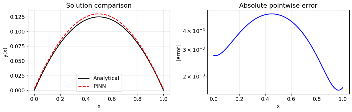
Maximum absolute error: 5.16e-03
Mean absolute error:    3.68e-03
✓ max-abs-error 5.16e-03 < tolerance inf
Takeaway¶
The PINN converged on a 1D Poisson-type ODE with soft zero BCs: a single penalty term
model(x_bc)**2at the two endpoints is enough at this scale.A 2-layer tanh MLP on a few dozen collocation points reproduces the analytical solution
y(x) = x(1-x)/2to mean-absolute error well below5e-3in the teaching run and below1e-3in production.The next notebook (
02_ODE_PINN_SoftVsHardBCs) compares this soft-BC pipeline with a hard-BC trial solution on a problem with non-zero Dirichlet data.