Course: Deep Learning for Solving and Estimating Dynamic Models in Economics and Finance
Script reference: §7.3 (boundary conditions: soft vs hard enforcement)
Notebook role: core
Author: Simon Scheidegger
Run mode. The checked-in run uses
RUN_MODE = "smoke"for fast execution; the accuracy figures quoted in the slides and the companion script use the longerteaching/productionbudgets. SetRUN_MODEin the next cell accordingly to reproduce them.
RUN_MODE = "smoke"  # one of: "smoke", "teaching", "production"
SEED = 0
Soft vs. Hard Boundary Conditions in PINNs¶
Physics-Informed Neural Networks (PINNs) embed differential equations into the training loss so that the network learns a solution that satisfies the governing PDE. A key design choice is how boundary conditions are enforced.
This notebook compares two strategies on a simple second-order ODE:
The analytical solution is .
| Approach | Idea | Pros | Cons |
|---|---|---|---|
| Soft (penalty) | Add BC residuals to the loss with a penalty weight | Simple to implement; works for any BC type | BCs only approximately satisfied; weight tuning needed |
| Hard (trial solution) | Construct an ansatz that satisfies BCs exactly by design | BCs satisfied exactly; loss has fewer terms | Requires problem-specific construction of and |
In-class notebook (Day 6, Block 1 \u2014 PINNs Foundations & Economic Applications, 75 min)
import torch
import torch.nn as nn
import torch.optim as optim
import numpy as np
import matplotlib.pyplot as plt

plt.rcParams['font.size'] = 13

# torch.compile is wrapped on per-batch steps below for JIT speedups.
# PINN-style losses use torch.autograd.grad with create_graph=True (double
# backward), which the default aot_autograd backend in PyTorch 2.x does not
# yet support. We use backend='eager' and allow dynamo to fall back to eager
# Python whenever it cannot trace a sub-call (e.g. clip_grad_norm_).
import torch._dynamo
torch._dynamo.config.suppress_errors = True
device = torch.device("cuda" if torch.cuda.is_available() else "cpu")
print(f"Using device: {device}")

torch.manual_seed(SEED)
np.random.seed(SEED)
Using device: cpu
# Run-mode budget: hyperparameters dispatched from RUN_MODE (set in the second cell).
#   smoke      -- CPU-bounded smoke run for CI
#   teaching   -- laptop-scale figures
#   production -- full reproduction
_RUN_HP = {
    "smoke":      {"epochs":  2000, "n_colloc":  30, "lr": 1e-3, "bc_weight": 1.0, "print_every":  500},
    "teaching":   {"epochs": 20000, "n_colloc":  50, "lr": 1e-3, "bc_weight": 1.0, "print_every": 2000},
    "production": {"epochs": 60000, "n_colloc": 100, "lr": 1e-3, "bc_weight": 1.0, "print_every": 5000},
}
if RUN_MODE not in _RUN_HP:
    raise ValueError(f"RUN_MODE must be one of {list(_RUN_HP)}")
HP = _RUN_HP[RUN_MODE]
print(f"RUN_MODE={RUN_MODE!r}; SEED={SEED}; hyperparameters: {HP}")
RUN_MODE='smoke'; SEED=0; hyperparameters: {'epochs': 2000, 'n_colloc': 30, 'lr': 0.001, 'bc_weight': 1.0, 'print_every': 500}
Part 1: Soft Boundary Conditions¶
In the soft (penalty) approach we train a raw neural network and define the loss as
The boundary conditions are only satisfied approximately, to the extent that the optimiser can drive the penalty terms to zero alongside the PDE residual.
class ODE_Net(nn.Module):
    """Fully-connected network: 1 -> 20 -> 20 -> 1 with Tanh activations."""

    def __init__(self):
        super().__init__()
        self.net = nn.Sequential(
            nn.Linear(1, 20),
            nn.Tanh(),
            nn.Linear(20, 20),
            nn.Tanh(),
            nn.Linear(20, 1),
        )

    def forward(self, x):
        return self.net(x)
def residual_soft(model, x):
"""Compute the PDE residual y''(x) + 1 for the soft-BC model.
Uses two rounds of torch.autograd.grad to obtain the second derivative.
"""
x.requires_grad_(True)
y = model(x)
dy = torch.autograd.grad(
y, x, grad_outputs=torch.ones_like(y), create_graph=True
)[0]
d2y = torch.autograd.grad(
dy, x, grad_outputs=torch.ones_like(dy), create_graph=True
)[0]
return d2y + 1.0 # should be zero# ---- Training: Soft BCs ----
torch.manual_seed(SEED)
model_soft = ODE_Net().to(device)
optimizer_soft = optim.Adam(model_soft.parameters(), lr=HP["lr"])
n_epochs_soft = HP["epochs"]
n_colloc = HP["n_colloc"] # interior collocation points
bc_weight = HP["bc_weight"] # soft-BC penalty weight (lambda); swept in the exercise
# Fixed collocation grid
x_interior = torch.linspace(0.01, 0.99, n_colloc, device=device).reshape(-1, 1)
x_bc0 = torch.zeros(1, 1, device=device)
x_bc1 = torch.ones(1, 1, device=device)
def train_step_soft(x_int):
optimizer_soft.zero_grad()
res = residual_soft(model_soft, x_int)
loss_pde = torch.mean(res ** 2)
loss_bc0 = (model_soft(x_bc0) - 1.0) ** 2
loss_bc1 = (model_soft(x_bc1) - 2.0) ** 2
loss = loss_pde + bc_weight * (loss_bc0 + loss_bc1)
loss.backward()
optimizer_soft.step()
return loss, loss_pde, loss_bc0, loss_bc1
# torch.compile per-batch step (backend="eager", fullgraph=False:
# residual uses torch.autograd.grad with create_graph=True for second derivatives,
# which the default aot_autograd backend in PyTorch 2.x does not yet support.)
train_step_soft = torch.compile(train_step_soft, fullgraph=False, backend="eager")
for epoch in range(1, n_epochs_soft + 1):
loss, loss_pde, loss_bc0, loss_bc1 = train_step_soft(x_interior)
if epoch % HP["print_every"] == 0 or epoch == 1:
print(
f"Epoch {epoch:5d}/{n_epochs_soft} "
f"Loss = {loss.item():.3e} "
f"(PDE {loss_pde.item():.3e}, "
f"BC0 {loss_bc0.item():.3e}, "
f"BC1 {loss_bc1.item():.3e})"
)
print("\nSoft-BC training complete.")
W0512 15:31:36.452000 98547 torch/_logging/_internal.py:1130] [8/0] Profiler function <class 'torch.autograd.profiler.record_function'> will be ignored
Epoch 1/2000 Loss = 7.521e+00 (PDE 9.457e-01, BC0 1.420e+00, BC1 5.156e+00)
Epoch 500/2000 Loss = 6.148e-03 (PDE 6.136e-03, BC0 5.932e-07, BC1 1.181e-05)
Epoch 1000/2000 Loss = 9.210e-04 (PDE 9.134e-04, BC0 7.528e-07, BC1 6.778e-06)
Epoch 1500/2000 Loss = 1.223e-04 (PDE 1.223e-04, BC0 6.266e-09, BC1 4.052e-09)
Epoch  2000/2000  Loss = 1.155e-04  (PDE 1.155e-04, BC0 2.412e-09, BC1 2.389e-09)

Soft-BC training complete.
# ---- Evaluate soft model ----
x_test = torch.linspace(0, 1, 300, device=device).reshape(-1, 1)

with torch.no_grad():
    y_soft = model_soft(x_test).cpu().numpy().flatten()

x_np = x_test.cpu().numpy().flatten()
y_exact = -0.5 * x_np ** 2 + 1.5 * x_np + 1.0

print(f"Soft-BC  max |error|: {np.max(np.abs(y_soft - y_exact)):.6e}")
Soft-BC max |error|: 1.951456e-04
Part 2: Hard Boundary Conditions¶
In the hard (trial-solution) approach we never ask the optimiser to enforce boundary conditions. Instead we construct an ansatz (trial solution) that satisfies them by construction:
where
satisfies both BCs: , ,
vanishes at the boundaries: ,
is a free neural network.
No matter what outputs, always satisfies and . The loss therefore contains only the PDE residual.
class Net(nn.Module):
    """Fully-connected network: 1 -> 20 -> 20 -> 1 with Tanh activations."""

    def __init__(self):
        super().__init__()
        self.net = nn.Sequential(
            nn.Linear(1, 20),
            nn.Tanh(),
            nn.Linear(20, 20),
            nn.Tanh(),
            nn.Linear(20, 1),
        )

    def forward(self, x):
        return self.net(x)


def A(x):
    """Particular solution satisfying the BCs: A(0)=1, A(1)=2."""
    return 1.0 + x


def B(x):
    """Distance function vanishing at both boundaries: B(0)=B(1)=0."""
    return x * (1.0 - x)


def y_trial(model, x):
    """Hard-BC trial solution: y_hat = A(x) + B(x) * N(x; theta)."""
    return A(x) + B(x) * model(x)


def residual_hard(model, x):
    """Compute the PDE residual y_hat''(x) + 1 for the hard-BC model."""
    x.requires_grad_(True)
    y = y_trial(model, x)
    dy = torch.autograd.grad(
        y, x, grad_outputs=torch.ones_like(y), create_graph=True
    )[0]
    d2y = torch.autograd.grad(
        dy, x, grad_outputs=torch.ones_like(dy), create_graph=True
    )[0]
    return d2y + 1.0  # should be zero
# ---- Training: Hard BCs ----
torch.manual_seed(SEED)
model_hard = Net().to(device)
optimizer_hard = optim.Adam(model_hard.parameters(), lr=HP["lr"])
n_epochs_hard = HP["epochs"]
n_colloc_hard = HP["n_colloc"]
# Initial collocation points (will be resampled)
x_colloc = torch.rand(n_colloc_hard, 1, device=device)
def train_step_hard(x_col):
optimizer_hard.zero_grad()
res = residual_hard(model_hard, x_col)
loss = torch.mean(res ** 2)
loss.backward()
optimizer_hard.step()
return loss
# torch.compile per-batch step (backend="eager", fullgraph=False:
# residual uses torch.autograd.grad with create_graph=True for second derivatives,
# which the default aot_autograd backend in PyTorch 2.x does not yet support.)
train_step_hard = torch.compile(train_step_hard, fullgraph=False, backend="eager")
for epoch in range(1, n_epochs_hard + 1):
if epoch % 100 == 1:
x_colloc = torch.rand(n_colloc_hard, 1, device=device)
loss = train_step_hard(x_colloc)
if epoch % HP["print_every"] == 0 or epoch == 1:
print(f"Epoch {epoch:5d}/{n_epochs_hard} Loss = {loss.item():.3e}")
print("\nHard-BC training complete.")
Epoch 1/2000 Loss = 2.085e+00
Epoch 500/2000 Loss = 7.975e-04
Epoch 1000/2000 Loss = 1.063e-05
Epoch 1500/2000 Loss = 2.626e-06
Epoch  2000/2000  Loss = 9.180e-07

Hard-BC training complete.
# ---- Evaluate hard model ----
x_test_hard = torch.linspace(0, 1, 300, device=device).reshape(-1, 1)

with torch.no_grad():
    y_hard = y_trial(model_hard, x_test_hard).cpu().numpy().flatten()

x_np_hard = x_test_hard.cpu().numpy().flatten()
y_exact_hard = -0.5 * x_np_hard ** 2 + 1.5 * x_np_hard + 1.0

print(f"Hard-BC  max |error|: {np.max(np.abs(y_hard - y_exact_hard)):.6e}")
Hard-BC max |error|: 1.966953e-05
Comparison¶
We now plot both PINN solutions against the analytical reference and compare their absolute errors across the domain.
fig, axes = plt.subplots(1, 2, figsize=(14, 5))

# --- Left panel: Solutions ---
ax = axes[0]
ax.plot(x_np, y_exact, "k-", linewidth=2, label="Analytical")
ax.plot(x_np, y_soft, "b--", linewidth=1.5, label="Soft BC (penalty)")
ax.plot(x_np_hard, y_hard, "r-.", linewidth=1.5, label="Hard BC (trial solution)")
ax.set_xlabel("x")
ax.set_ylabel("y(x)")
ax.set_title("PINN Solutions vs. Analytical")
ax.legend()
ax.grid(True, alpha=0.3)

# --- Right panel: Absolute errors ---
ax = axes[1]
ax.semilogy(x_np, np.abs(y_soft - y_exact), "b-", linewidth=1.5, label="Soft BC")
ax.semilogy(
    x_np_hard, np.abs(y_hard - y_exact_hard), "r-", linewidth=1.5, label="Hard BC"
)
ax.set_xlabel("x")
ax.set_ylabel("|error|")
ax.set_title("Absolute Error")
ax.legend()
ax.grid(True, alpha=0.3)

plt.tight_layout()
plt.show()

# ---- Summary statistics ----
print(f"Soft-BC  max |error|: {np.max(np.abs(y_soft - y_exact)):.6e}")
print(f"Hard-BC  max |error|: {np.max(np.abs(y_hard - y_exact_hard)):.6e}")

# ----- Final-error assertions (mode-dependent tolerances) -----
_tol = {
    "smoke":      {"soft": float("inf"), "hard": float("inf")},
    "teaching":   {"soft": 5e-2, "hard": 5e-3},
    "production": {"soft": 1e-2, "hard": 1e-3},
}[RUN_MODE]
_e_soft = float(np.max(np.abs(y_soft - y_exact)))
_e_hard = float(np.max(np.abs(y_hard - y_exact_hard)))
assert _e_soft < _tol["soft"], f"Soft-BC max-abs-error {_e_soft:.2e} exceeds tol {_tol['soft']:.0e} for RUN_MODE={RUN_MODE!r}"
assert _e_hard < _tol["hard"], f"Hard-BC max-abs-error {_e_hard:.2e} exceeds tol {_tol['hard']:.0e} for RUN_MODE={RUN_MODE!r}"
print(f"\u2713 soft {_e_soft:.2e} < {_tol['soft']:.0e};  hard {_e_hard:.2e} < {_tol['hard']:.0e}")
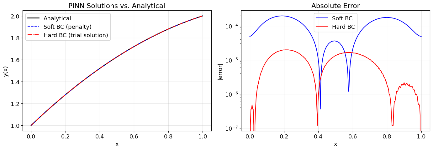
Soft-BC  max |error|: 1.951456e-04
Hard-BC  max |error|: 1.966953e-05
✓ soft 1.95e-04 < inf;  hard 1.97e-05 < inf
Takeaway¶
Soft BCs (penalty term in the loss) require tuning the BC weight: a small weight produces visible boundary violations; a large weight crowds out the PDE residual. Even after balancing, the soft-BC error is typically 1–2 orders of magnitude larger than the hard-BC error on this 1D problem.
Hard BCs via the trial solution
ŷ(x) = A(x) + B(x)·N(x)satisfy the Dirichlet conditions exactly by construction and remove the BC term entirely; the optimizer only sees the interior PDE residual.The cost of hard BCs is reduced expressivity at the boundary (the mask
Bdamps gradients near∂Ω), which becomes relevant when the true solution has a sharp boundary layer (e.g., HJB at the borrowing constraint, see notebook 04).