Course: Deep Learning for Solving and Estimating Dynamic Models in Economics and Finance
Script reference: §6.7 (Sequence-space DEQNs) -- JAX/optax port of the upstream pedagogical KS tutorial
Notebook role: extension
Author: Simon Scheidegger (course adaptation; upstream attribution preserved below)
# Run-mode switch (smoke = CPU-bounded for CI, teaching = laptop figures, production = full reproduction).
RUN_MODE = "smoke"  # one of: "smoke", "teaching", "production"
SEED = 0
Upstream attribution¶
This notebook is a JAX/optax port of the upstream pedagogical tutorial 01_KrusellSmith_Tutorial_CPU.ipynb released with the paper Deep Learning in the Sequence Space by Marlon Azinovic-Yang and Jan \v{Z}emli\v{c}ka (arXiv:2509.13623).
Upstream repository: https://
github .com /azinoma /DeepLearningInTheSequenceSpace Paper: Azinovic-Yang & \v{Z}emli\v{c}ka (2025), arXiv:2509.13623
The course adaptation only adds (i) a TUTORIAL_MODE switch derived from the kit-mandated RUN_MODE, (ii) an explicit shape-guarantee diagnostic, and (iii) clarifying inline commentary. The mathematics and the algorithm are unchanged from the upstream tutorial.
Recommended workflow¶
The default
RUN_MODE = "smoke"(cell 1) maps toTUTORIAL_MODE = "quick"so the notebook runs in a few minutes on a laptop CPU.Setting
RUN_MODE = "production"switches toTUTORIAL_MODE = "full"for the larger, slower run.If the import cell complains about missing packages, install them with
pip install jax optax scipy matplotliband rerun.
Note on
K_ss. The deterministic representative-agent benchmarkK_ssdefined below is a convenient reference point for plots and initial conditions. It is not the stochastic heterogeneous-agent equilibrium capital stock.
import jax
import jax.numpy as jnp
from jax import lax
import matplotlib.pyplot as plt
import numpy as np
import optax
from scipy.interpolate import BSpline

print(f"JAX version: {jax.__version__}")
print(f"Devices: {jax.devices()}")

# Derived from the kit-mandated RUN_MODE in cell 1.
TUTORIAL_MODE = "full" if RUN_MODE == "production" else "quick"
assert TUTORIAL_MODE in {"quick", "full"}
print(f"Tutorial mode: {TUTORIAL_MODE}")
JAX version: 0.6.2
Devices: [CpuDevice(id=0)]
Tutorial mode: quick
Part 1: The Economic Model¶
The Krusell-Smith Economy¶
We consider an economy with:
A continuum of households who save and consume
Aggregate risk: productivity follows a Markov chain
Idiosyncratic risk: each household’s efficiency also follows a Markov chain
Prices¶
A representative firm uses Cobb-Douglas technology , giving:
Household Problem¶
Each household chooses consumption to maximize:
subject to:
Optimality Conditions¶
At an interior solution (), the Euler equation holds:
At the borrowing constraint (), the Euler gap can be nonzero, but the Kuhn-Tucker conditions still have to hold.
For teaching purposes, this notebook keeps the Markov structure deliberately simple: both aggregate and idiosyncratic shocks have two states.
Calibration¶
Let’s set up the model parameters:
#===Model Parameters===
ALPHA = 0.36   # capital share
DELTA = 0.025  # depreciation
BETA = 0.93    # discount factor (log utility is hardcoded throughout)

# Idiosyncratic shocks: low and high efficiency
EPS_VALS = jnp.array([0.5, 1.5])
PI_EPS = jnp.array([[0.9, 0.1],  # P(eps'=L | eps=L) = 0.9
                     [0.1, 0.9]]) # P(eps'=H | eps=H) = 0.9

# Aggregate shocks: low and high productivity
Z_VALS = jnp.array([0.93, 1.07])
PI_Z = jnp.array([[0.7, 0.3],  # persistence = 0.7
                  [0.3, 0.7]])

N_EPS = len(EPS_VALS)
N_Z = len(Z_VALS)

# Steady-state capital (from the deterministic Euler equation)
R_ss = 1.0 / BETA
K_ss = ((R_ss - 1.0 + DELTA) / ALPHA) ** (1.0 / (ALPHA - 1.0))
print(f"Steady-state capital: K_ss = {K_ss:.2f}")

# Price functions
def compute_prices(K, L, Z):
    """
    Cobb-Douglas factor prices.
    """
    KL = K / L
    R = 1.0 - DELTA + ALPHA * Z * KL ** (ALPHA - 1.0)
    w = (1.0 - ALPHA) * Z * KL ** ALPHA
    return R, w
Steady-state capital: K_ss = 7.37
Part 2: The I-Spline MPC Representation¶
Shape preserving operator learning¶
For a given aggregate history of shocks, , we want to predict a consumption function . Following the operator learning idea, we want to predict the consumption values on a grid of idisyncratic states, and then use piecewise linear interpolation inbetween.
We want a consumption function that is:
Increasing in (richer people consume more)
Concave in (the marginal propensity to consume decreases with wealth)
Feasible: (no borrowing, positive consumption)
Instead of parameterizing directly, we parameterize the marginal propensity to consume (MPC) — how much of each extra dollar of wealth gets consumed:
where:
: MPC at the borrowing constraint (from a sigmoid)
: I-spline basis functions (monotonically increasing from 0 to 1)
: weights from a “phantom-zero” softmax
Since each is increasing and , the MPC is decreasing by construction. Since , the MPC is positive everywhere. Since , consumption is feasible.
We then recover consumption by cumulation on a fixed grid:
Let’s build it step by step.¶
Step 2a: The Capital Grid¶
We use a log-spaced grid to get more resolution near where the policy is steepest:
# === Capital Grid ===
GRID_CONFIG = {
    "quick": {"N": 60, "K_MAX": 60.0},
    "full": {"N": 100, "K_MAX": 100.0},
}[TUTORIAL_MODE]

N = GRID_CONFIG["N"]          # number of intervals (N+1 grid points)
K_MAX = GRID_CONFIG["K_MAX"]  # upper bound on capital

K_GRID_SHIFT = 0.5
BASIS_SHIFT = 0.5

x_grid = np.linspace(np.log(K_GRID_SHIFT), np.log(K_MAX + K_GRID_SHIFT), N + 1)
k_grid = jnp.array(np.exp(x_grid) - K_GRID_SHIFT)
dk = jnp.diff(k_grid)
x0 = float(x_grid[0])
delta_x = float((x_grid[-1] - x_grid[0]) / N)

# Visualize the grid spacing
fig, ax = plt.subplots(figsize=(10, 2))
ax.scatter(np.asarray(k_grid), np.zeros(N + 1), s=6, alpha=0.7)
ax.set_xlabel("Capital ")
ax.set_title(f"Log-spaced grid: {N+1} points in [0, {K_MAX}]")
ax.set_yticks([])
ax.axvline(K_ss, color='red', linestyle='--', alpha=0.5, label=f"deterministic $K_{{ss}}={K_ss:.1f}$")
ax.legend()
plt.tight_layout()
plt.show()
print(f"Grid spacing: {float(dk[0]):.3f} (near k=0) to {float(dk[-1]):.1f} (near k_max)")
Grid spacing: 0.042 (near k=0) to 4.6 (near k_max)
Step 2b: I-Spline Basis Functions¶
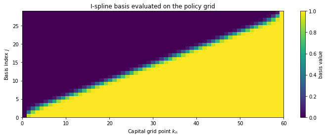
It helps to separate the grid from the basis.
The policy grid
k_grid = (k_0,\dots,k_N)tells us where we store the policy.The I-spline basis tells us how we parameterize the shape of the MPC on that grid.
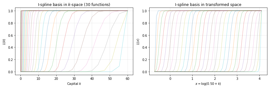
We build cubic I-splines in the transformed coordinate
The spline knots live in this x-space; they are not the same as the points in k_grid.
After constructing the basis functions , we evaluate each one at every grid point
So ispline_basis is a matrix :
rows = basis functions, columns = capital grid points.
Each I-spline is a smooth cumulative switch: it starts near 0, rises over a local region, and ends near 1.
Because each is increasing, any nonnegative weighted sum of them is also increasing.
The neural network outputs, for each income state:
a boundary MPC
nonnegative weights with
These define the MPC on the grid:
Since the weighted sum increases with , the MPC decreases with .
That gives us concavity by construction.
We then recover consumption on the grid by discrete integration:
A crucial point: the splines are used to construct the MPC values on the grid.
Off the grid, the notebook does not use spline interpolation of ; it uses simple piecewise-linear interpolation of c_grid.
# === Build I-Spline Basis ===
N_INTERIOR = 26 if TUTORIAL_MODE == "quick" else 56
ORDER = 4           # cubic I-splines

def build_ispline_basis(k_grid, n_interior=56, order=4, basis_shift=None):
    """Precompute I-spline basis at the grid points."""
    if basis_shift is None:
        basis_shift = BASIS_SHIFT
    k_arr = np.asarray(k_grid)
    x = np.log(basis_shift + k_arr)
    x_min, x_max = float(x[0]), float(x[-1])

    # Equidistant interior knots in x-space
    knots_int = np.linspace(x_min, x_max, n_interior + 2)[1:-1]
    knots = np.concatenate([np.repeat(x_min, order), knots_int, np.repeat(x_max, order)])
    n_basis = len(knots) - order

    # Compute I-splines (= integral of B-splines)
    basis = np.zeros((n_basis, len(k_arr)))
    for idx in range(n_basis):
        c = np.zeros(n_basis)
        c[idx] = 1.0
        bspl = BSpline(knots, c, order - 1, extrapolate=False)
        t_span = knots[idx + order] - knots[idx]
        if t_span < 1e-12:
            continue
        anti = bspl.antiderivative()
        basis[idx] = (order / t_span) * np.nan_to_num(anti(x) - anti(x_min), 0.0)

    return jnp.array(np.clip(basis, 0.0, 1.0))

ispline_basis = build_ispline_basis(k_grid, N_INTERIOR, ORDER, basis_shift=BASIS_SHIFT)
J = ispline_basis.shape[0]
print(f"Built {J} I-spline basis functions on {N+1} grid points")


# What the basis matrix actually is
B = np.asarray(ispline_basis)
print("Basis matrix shape:", B.shape)
print(f"Entry B[j, n] = I_j(log({BASIS_SHIFT:.2f} + k_grid[n]))")

fig, ax = plt.subplots(figsize=(10, 4))
im = ax.imshow(
    B,
    aspect='auto',
    origin='lower',
    extent=[float(k_grid[0]), float(k_grid[-1]), 0, B.shape[0]-1]
)
ax.set_xlabel("Capital grid point $k_n$")
ax.set_ylabel("Basis index $j$")
ax.set_title("I-spline basis evaluated on the policy grid")
fig.colorbar(im, ax=ax, label="basis value")
plt.tight_layout()
plt.show()


fig, axes = plt.subplots(1, 2, figsize=(12, 4))
for j in range(J):
    axes[0].plot(np.asarray(k_grid), np.asarray(ispline_basis[j]), linewidth=0.8, alpha=0.5)
axes[0].set_xlabel("Capital $k$")
axes[0].set_ylabel("$I_j(k)$")
axes[0].set_title(f"I-spline basis in $k$-space ({J} functions)")
axes[0].grid(True, alpha=0.3)

x_vals = np.log(BASIS_SHIFT + np.asarray(k_grid))
for j in range(J):
    axes[1].plot(x_vals, np.asarray(ispline_basis[j]), linewidth=0.8, alpha=0.5)
axes[1].set_xlabel(rf"$x = \log({BASIS_SHIFT:.2f} + k)$")
axes[1].set_ylabel("$I_j(x)$")
axes[1].set_title("I-spline basis in transformed space")
axes[1].grid(True, alpha=0.3)

plt.tight_layout()
plt.show()
Built 30 I-spline basis functions on 61 grid points
Basis matrix shape: (30, 61)
Entry B[j, n] = I_j(log(0.50 + k_grid[n]))
Step 2c: The Neural Network Actor¶
The actor is a simple 2-layer MLP that maps a short history of aggregate shocks to I-spline coefficients.
This is a practical approximation to the Krusell-Smith idea that the wealth distribution can often be summarized well by a low-dimensional object. Here we use a finite shock history rather than claiming that the full distribution is literally a function of the last shocks.
# === Neural Network Actor ===
H = 50            # history length (last H aggregate shocks)
HIDDEN_DIM = 64   # MLP hidden layer width
INPUT_DIM = H * (N_Z + 1)  # one-hot + value per lag

def init_actor(key, input_dim, hidden_dim, n_eps, J):
    """Initialize a 2-hidden-layer MLP."""
    k1, k2, k3 = jax.random.split(key, 3)
    output_dim = n_eps * (1 + J)  # per eps: 1 alpha logit + J weight logits
    return {
        "W_0": jnp.sqrt(2.0/input_dim) * jax.random.normal(k1, (input_dim, hidden_dim)),
        "b_0": jnp.zeros(hidden_dim),
        "W_1": jnp.sqrt(2.0/hidden_dim) * jax.random.normal(k2, (hidden_dim, hidden_dim)),
        "b_1": jnp.zeros(hidden_dim),
        "W_2": 0.01 * jax.random.normal(k3, (hidden_dim, output_dim)),
        "b_2": jnp.zeros(output_dim),
    }

def actor_c_grid(psi, agg_input, R, w):
    """Forward pass: aggregate input -> consumption on the k-grid.

    Returns: c_grid of shape (n_eps, N+1)
    """
    # MLP forward pass (tanh activation — sweep-validated, 3x better than relu)
    h = jnp.tanh(agg_input @ psi["W_0"] + psi["b_0"])
    h = jnp.tanh(h @ psi["W_1"] + psi["b_1"])
    raw = (h @ psi["W_2"] + psi["b_2"]).reshape(N_EPS, 1 + J)

    # Boundary MPC: sigmoid -> (0, 1)
    alpha = jax.nn.sigmoid(raw[:, 0])                        # (n_eps,)

    # Phantom-zero softmax: guarantees weights >= 0 and sum < 1
    logits = raw[:, 1:]                                       # (n_eps, J)
    augmented = jnp.concatenate([jnp.zeros((N_EPS, 1)), logits], axis=1)
    w_tilde = jax.nn.softmax(augmented, axis=1)[:, 1:]       # (n_eps, J)

    # MPC on the grid: alpha * (1 - weighted I-splines)
    mpc = alpha[:, None] * (1.0 - w_tilde @ ispline_basis)   # (n_eps, N+1)

    # Cumulate consumption on the grid from the MPC schedule.
    # Boundary: c(k_0) = MPC(k_0) · m(k_0), where m = wε + Rk is cash-on-hand
    c0 = mpc[:, 0] * (w * EPS_VALS + R * k_grid[0])
    # Increments: Δc_n = MPC(k_n) · R · Δk_n — each MPC value used exactly once
    dc = mpc[:, 1:] * (R * dk[None, :])
    c_grid = jnp.concatenate([c0[:, None], c0[:, None] + jnp.cumsum(dc, axis=1)], axis=1)
    return c_grid

# Initialize and check
key = jax.random.PRNGKey(0)
key, init_key = jax.random.split(key)
psi = init_actor(init_key, INPUT_DIM, HIDDEN_DIM, N_EPS, J)
n_params = sum(p.size for p in jax.tree_util.tree_leaves(psi))
print(f"Actor parameters: {n_params}")
print(f"Input dim: {INPUT_DIM} (H={H} x {N_Z+1} features per lag)")
print(f"Output dim: {N_EPS} x (1 + {J}) = {N_EPS * (1 + J)}")
Actor parameters: 17854
Input dim: 150 (H=50 x 3 features per lag)
Output dim: 2 x (1 + 30) = 62
Let’s visualize what the initial (random) policy looks like. Even before training, the shape guarantees hold:
# === Visualize Initial Policy ===
def encode_Z_history(z_hist):
    """Encode Z-history as one-hot + values."""
    onehot = jax.nn.one_hot(z_hist, N_Z).reshape(-1)
    values = Z_VALS[z_hist].reshape(-1)
    return jnp.concatenate([onehot, values])

def shape_report(c_grid, R, w, title):
    """Verify the four shape guarantees of the I-spline MPC policy.

    Checks (all should hold by construction):
      min Δc >= 0        — consumption is increasing in k
      max(c - m) <= 0    — consumption is feasible (c ≤ cash-on-hand)
      MPC ∈ [0, 1]       — marginal propensity in valid range
      max ΔMPC <= 0      — MPC is decreasing (consumption is concave)
    """
    m_grid = float(w) * np.asarray(EPS_VALS)[:, None] + float(R) * k_np[None, :]
    min_dc = float(np.min(np.diff(c_grid, axis=1)))
    max_excess = float(np.max(c_grid - m_grid))
    mpc_intervals = np.diff(c_grid, axis=1) / (float(R) * np.asarray(dk)[None, :])
    min_mpc = float(np.min(mpc_intervals))
    max_mpc = float(np.max(mpc_intervals))
    max_upturn = float(np.max(np.diff(mpc_intervals, axis=1)))
    print(f"Shape check for {title}:")
    print(f"  min Δc across grid intervals      = {min_dc: .3e}  (should be >= 0)")
    print(f"  max(c - cash on hand)             = {max_excess: .3e}  (should be <= 0)")
    print(f"  MPC range on intervals            = [{min_mpc: .3f}, {max_mpc: .3f}]")
    print(f"  max increase in MPC across k-grid = {max_upturn: .3e}  (should be <= 0)")

# Use a constant Z=Z_L history for visualization
z_hist_dummy = jnp.zeros(H, dtype=jnp.int32)
agg_input = encode_Z_history(z_hist_dummy)
R_vis, w_vis = compute_prices(K_ss, 1.0, float(Z_VALS[0]))
c_grid_init = np.asarray(actor_c_grid(psi, agg_input, float(R_vis), float(w_vis)))

k_np = np.asarray(k_grid)
fig, axes = plt.subplots(1, 2, figsize=(12, 4))
colors = ["#1f77b4", "#ff7f0e"]
labels = [r"$\varepsilon_L$", r"$\varepsilon_H$"]

for e in range(N_EPS):
    m = float(w_vis) * float(EPS_VALS[e]) + float(R_vis) * k_np
    axes[0].plot(k_np, c_grid_init[e], color=colors[e], label=labels[e])
    axes[0].plot(k_np, m, color=colors[e], linestyle=':', alpha=0.3, label=f"$m$ ({labels[e]})")

    # MPC at k=0: consumption as fraction of cash-on-hand (= boundary MPC α)
    mpc = np.zeros_like(k_np)
    mpc[0] = c_grid_init[e, 0] / max(m[0], 1e-10)
    # MPC at k>0: finite-difference Δc/Δm = Δc/(R·Δk), matches I-spline MPC by construction
    mpc[1:] = np.diff(c_grid_init[e]) / (float(R_vis) * np.asarray(dk))
    axes[1].plot(k_np, mpc, color=colors[e], label=labels[e])

axes[0].set_xlabel("Capital $k$")
axes[0].set_ylabel("Consumption $c$")
axes[0].set_title("Initial policy (random weights)")
axes[0].legend(fontsize=8)
axes[0].grid(True, alpha=0.3)
axes[1].set_xlabel("Capital $k$")
axes[1].set_ylabel("MPC")
axes[1].set_title("MPC (decreasing by construction)")
axes[1].set_ylim(-0.05, 1.05)
axes[1].grid(True, alpha=0.3)
axes[1].legend(fontsize=8)
plt.tight_layout()
plt.show()

shape_report(c_grid_init, float(R_vis), float(w_vis), "initial random policy")
print("Even before training, the grid policy is increasing, feasible, and concave by construction.")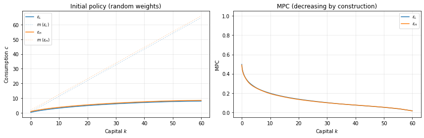
Shape check for initial random policy:
  min Δc across grid intervals      =  2.084e-02  (should be >= 0)
  max(c - cash on hand)             = -3.068e-01  (should be <= 0)
  MPC range on intervals            = [ 0.016,  0.476]
  max increase in MPC across k-grid = -6.322e-03  (should be <= 0)
Even before training, the grid policy is increasing, feasible, and concave by construction.
Part 3: Simulation with Young’s (2010) Non-Stochastic Method¶
To evaluate the Euler equation we need aggregate capital and labor , which depend on the cross-sectional wealth distribution. Instead of simulating a panel of individual households (Monte Carlo), we track the full distribution as a histogram on the grid.
Each period, for every grid point :
Compute next-period capital:
generally falls between two grid points. Split the mass to the two neighbors proportionally (lottery).
Apply the idiosyncratic transition matrix across income states.
Key advantage: aggregates and are exact weighted sums — no sampling noise. This eliminates the Monte Carlo noise floor (~10-6) that limits accuracy with household panels.
The replay buffer stores coupled pairs of (Z-history, distribution ). Each epoch we sample states, simulate forward periods, and store the terminal distributions.
# === Simulation: Young (2010) Non-Stochastic Method ===
SIM_CONFIG = {
    "quick": {"T": 100, "N_AGG": 8, "BUFFER_CAP": 128},
    "full":  {"T": 100, "N_AGG": 8, "BUFFER_CAP": 128},
}[TUTORIAL_MODE]

T = SIM_CONFIG["T"]
N_AGG = SIM_CONFIG["N_AGG"]
BUFFER_CAP = SIM_CONFIG["BUFFER_CAP"]

def interpolate(vals_grid, eps_idx, k):
    """Piecewise-linear interpolation on the k-grid."""
    x = jnp.log(K_GRID_SHIFT + k)
    j = jnp.clip(jnp.floor((x - x0) / delta_x).astype(jnp.int32), 0, N - 1)
    w_lo = (k_grid[j + 1] - k) / (k_grid[j + 1] - k_grid[j])
    return w_lo * vals_grid[eps_idx, j] + (1.0 - w_lo) * vals_grid[eps_idx, j + 1]

def draw_Z_path(key, T, z_init):
    """Draw T aggregate shocks. Returns (emitted_path, terminal_carry).

    emitted_path = [z_t, z_{t+1}, ..., z_{t+T-1}],
    terminal_carry = z_{t+T}.
    """
    keys = jax.random.split(key, T)
    def step(z, k):
        z_next = (jax.random.uniform(k) >= PI_Z[z, 0]).astype(jnp.int32)
        return z_next, z
    z_terminal, Z_path = lax.scan(step, z_init, keys)
    return Z_path, z_terminal

def make_agg_inputs(full_Z_seq, H, T):
    """Build encoded Z-history inputs for each simulation step."""
    offsets = jnp.arange(T)[:, None] + jnp.arange(H)[None, :]
    windows = full_Z_seq[offsets]
    return jax.vmap(encode_Z_history)(windows)

# --- Young (2010) distribution functions ---

def distribution_aggregates(mu):
    """Compute aggregate K and L from distribution mu(eps, k).

    mu has shape (N_EPS, N+1) and sums to 1.
    K = Σ k · μ(ε,k),  L = Σ ε · μ(ε,k).
    """
    K = jnp.sum(mu * k_grid[None, :])
    L = jnp.sum(mu * EPS_VALS[:, None])
    return jnp.maximum(K, 0.01), jnp.maximum(L, 0.01)

def distribution_step(mu, c_grid_t, R, w):
    """Advance the distribution one period (Young 2010).

    For each (eps, k) grid point:
      1. Compute next-period capital: k' = w·eps + R·k - c(eps, k)
      2. Find the two neighboring grid points around k'
      3. Split the mass to those neighbors (lottery)
      4. Apply the idiosyncratic transition matrix Pi_eps

    Args:
        mu:        (N_EPS, N+1) current distribution, sums to 1
        c_grid_t:  (N_EPS, N+1) consumption policy on the grid
        R, w:      current factor prices
    Returns:
        mu_next:   (N_EPS, N+1) next-period distribution
    """
    # Next-period capital for every (eps, k) grid point
    m_grid = w * EPS_VALS[:, None] + R * k_grid[None, :]
    k_next = jnp.clip(m_grid - c_grid_t, 0.0, k_grid[-1])

    # Find grid position of k' in log-space
    x_next = jnp.log(K_GRID_SHIFT + k_next)
    j_lo = jnp.clip(
        jnp.floor((x_next - x0) / delta_x).astype(jnp.int32), 0, N - 1)

    # Lottery weights: fraction of mass going to lower vs upper neighbor
    k_lo = k_grid[j_lo]
    k_hi = k_grid[j_lo + 1]
    w_lo = (k_hi - k_next) / jnp.maximum(k_hi - k_lo, 1e-12)
    w_hi = 1.0 - w_lo

    # Scatter mass to neighboring grid points for each eps state
    def scatter_one_eps(i):
        mass = mu[i]                    # (N+1,)
        j = j_lo[i]                     # (N+1,) integer indices
        result = jnp.zeros(N + 1)
        result = result.at[j].add(mass * w_lo[i])
        result = result.at[j + 1].add(mass * w_hi[i])
        return result

    mu_after = jax.vmap(scatter_one_eps)(jnp.arange(N_EPS))   # (N_EPS, N+1)

    # Apply idiosyncratic transition: mu_next[i'] = Σ_i Pi[i, i'] · mu_after[i]
    mu_next = PI_EPS.T @ mu_after
    return mu_next

def initial_distribution(K_target):
    """Create an initial distribution centered around K_target.

    eps: uniform across states; k: Gaussian around K_target.
    Returns mu of shape (N_EPS, N+1), summing to 1.
    """
    eps_weight = jnp.ones(N_EPS) / N_EPS
    sigma_k = K_target * 0.3
    density = jnp.exp(-0.5 * ((k_grid - K_target) / sigma_k) ** 2)
    density = density / jnp.sum(density)
    mu = eps_weight[:, None] * density[None, :]
    return mu / jnp.sum(mu)

def simulate_young(psi, mu_init, Z_path, agg_inputs):
    """Simulate T periods using Young's non-stochastic method.

    Instead of tracking individual households, evolves the full
    distribution mu(eps, k) on the grid. Aggregates K, L are exact
    weighted sums — no Monte Carlo sampling noise.

    Args:
        mu_init:    (N_EPS, N+1) initial distribution
        Z_path:     (T,) aggregate shock indices
        agg_inputs: (T, INPUT_DIM) encoded Z-histories
    Returns:
        mu_final:   (N_EPS, N+1) terminal distribution
    """
    def step(mu, inputs):
        Z_idx, agg_input_t = inputs
        K_t, L_t = distribution_aggregates(mu)
        K_t = jax.lax.stop_gradient(K_t)
        L_t = jax.lax.stop_gradient(L_t)
        R_t, w_t = compute_prices(K_t, L_t, Z_VALS[Z_idx])
        c_grid_t = actor_c_grid(psi, agg_input_t, R_t, w_t)
        mu_next = distribution_step(mu, c_grid_t, R_t, w_t)
        return mu_next, None

    mu_final, _ = lax.scan(step, mu_init, (Z_path, agg_inputs))
    return mu_final

print(f"Simulation config: T={T}, n_agg={N_AGG}, buffer={BUFFER_CAP}")
print("Using Young (2010) non-stochastic method — no MC noise in aggregates.")
Simulation config: T=100, n_agg=8, buffer=128
Using Young (2010) non-stochastic method — no MC noise in aggregates.
Part 4: The Fischer-Burmeister Loss¶
Why focus on Euler / KKT conditions?¶
In practice, directly maximizing discounted utility often gives weaker Euler-equation accuracy than directly training on the first-order conditions. In this notebook we therefore target the Euler / KKT residual itself.
The Fischer-Burmeister function¶
The household’s optimality has two cases:
Interior (): Euler equation holds with equality, i.e. where
Constrained (): Euler gap
The Fischer-Burmeister function encodes both in one smooth formula:
where is the relative savings slack.
For log utility, , so .
if and only if the KKT conditions are satisfied: either (interior) or (constrained).
# === Fischer-Burmeister Loss ===

def fb_loss_one_state(psi, z_history, mu):
    """Compute mean FB² on the full (eps, k) grid for one replay state.

    With Young's method, aggregates K, L come from the distribution mu
    (exact weighted sums). Next-period aggregates come from advancing
    mu one step with distribution_step — deterministic, no MC noise.
    """
    z_t = z_history[-1]

    # Current prices from distribution (exact aggregates)
    K_t, L_t = distribution_aggregates(mu)
    K_t, L_t = jax.lax.stop_gradient(K_t), jax.lax.stop_gradient(L_t)
    R_t, w_t = compute_prices(K_t, L_t, Z_VALS[z_t])
    R_t, w_t = jax.lax.stop_gradient(R_t), jax.lax.stop_gradient(w_t)

    # Current policy on the full grid
    agg_input = encode_Z_history(z_history)
    c_grid_t = actor_c_grid(psi, agg_input, R_t, w_t)

    # Next-period capital for each (eps, k) on the grid
    m_grid = w_t * EPS_VALS[:, None] + R_t * k_grid[None, :]
    k_next_grid = jnp.clip(m_grid - c_grid_t, 0.0, k_grid[-1])

    # Next-period aggregates from Young step (exact, deterministic)
    mu_next = distribution_step(mu, c_grid_t, R_t, w_t)
    K_next, L_next = distribution_aggregates(mu_next)
    K_next, L_next = jax.lax.stop_gradient(K_next), jax.lax.stop_gradient(L_next)

    # Continuation value: q = E[β R' u'(c')]
    # Outer loop over next-Z unrolled at trace time; inner eps vectorized.
    q = jnp.zeros_like(c_grid_t)
    for z_next in range(N_Z):
        z_hist_next = jnp.concatenate([z_history[1:], jnp.array([z_next])])
        agg_next = encode_Z_history(z_hist_next)
        R_next, w_next = compute_prices(K_next, L_next, Z_VALS[z_next])
        R_next, w_next = jax.lax.stop_gradient(R_next), jax.lax.stop_gradient(w_next)
        c_grid_next = actor_c_grid(psi, agg_next, R_next, w_next)

        # Vectorized next-eps integration
        def _interp_next(i_next):
            k_flat = k_next_grid.ravel()
            idx = jnp.full(k_flat.shape, i_next, dtype=jnp.int32)
            return interpolate(c_grid_next, idx, k_flat).reshape(N_EPS, N + 1)

        c_next_all = jax.vmap(_interp_next)(jnp.arange(N_EPS))
        mu_u = 1.0 / jnp.maximum(c_next_all, 1e-10)       # u'(c) = 1/c
        exp_uc = jnp.einsum('ij,jik->ik', PI_EPS, mu_u)
        q += PI_Z[z_t, z_next] * BETA * R_next * exp_uc

    # Euler-implied consumption and FB residual
    c_euler = 1.0 / jnp.maximum(q, 1e-10)
    c_scale = jnp.maximum(c_grid_t, 1e-10)
    g = (c_euler - c_grid_t) / c_scale          # relative Euler gap
    s = k_next_grid / c_scale                    # relative slack
    fb = jnp.sqrt(g**2 + s**2 + 1e-12) - g - s  # Fischer-Burmeister residual

    return jnp.mean(fb**2)

def fb_loss(psi, buf_z, buf_mu):
    """Mean FB² over all buffer states."""
    fb2_all = jax.vmap(lambda z, mu: fb_loss_one_state(psi, z, mu))(buf_z, buf_mu)
    return jnp.mean(fb2_all)

print("FB loss defined. With Young's method, aggregates are exact — no MC noise.")
FB loss defined. With Young's method, aggregates are exact — no MC noise.
Part 5: Training¶
Now we put everything together. Each epoch:
Sample replay states from the buffer
Simulate forward to evolve the buffer (no gradients needed here)
Take several FB gradient steps on the full buffer
The most important knob is the number of FB steps per buffer refresh. In quick mode we keep it smaller so the notebook runs fast.
# === Training Setup ===
# Hyperparameters from the sweep leaderboard (fastest to FB² < 1e-6):
# MLP 2×64 tanh, fb_batch=16, fb_steps=10, lr=5e-5, H=50, T=100
TRAIN_CONFIG = {
    "quick": {"LR": 5e-5, "FB_STEPS": 10, "FB_BATCH": 16, "N_EPOCHS": 5000,  "LOG_EVERY": 100},
    "full":  {"LR": 5e-5, "FB_STEPS": 10, "FB_BATCH": 16, "N_EPOCHS": 10_000, "LOG_EVERY": 200},
}[TUTORIAL_MODE]

LR = TRAIN_CONFIG["LR"]
FB_STEPS = TRAIN_CONFIG["FB_STEPS"]
FB_BATCH = TRAIN_CONFIG["FB_BATCH"]      # mini-batch size for FB gradient steps
N_EPOCHS = TRAIN_CONFIG["N_EPOCHS"]
LOG_EVERY = TRAIN_CONFIG["LOG_EVERY"]

optimizer = optax.chain(optax.clip_by_global_norm(1.0), optax.adam(LR))
opt_state = optimizer.init(psi)

@jax.jit
def fb_update(psi, opt_state, buf_z, buf_mu):
    loss, grads = jax.value_and_grad(fb_loss)(psi, buf_z, buf_mu)
    updates, new_opt = optimizer.update(grads, opt_state)
    new_psi = optax.apply_updates(psi, updates)
    return new_psi, new_opt, loss

@jax.jit
def run_simulations(key, psi, z_hists, mu_starts, z_inits):
    """Generate shocks, simulate distributions forward, return terminal states."""
    key, k1 = jax.random.split(key)
    z_keys = jax.random.split(k1, N_AGG)
    Z_paths, Z_terms = jax.vmap(lambda k, z0: draw_Z_path(k, T, z0))(z_keys, z_inits)

    full_Z = jnp.concatenate([z_hists, Z_paths[:, 1:]], axis=1)
    agg_inputs = jax.vmap(lambda seq: make_agg_inputs(seq, H, T))(full_Z)

    def sim1(mu, zp, ai):
        return simulate_young(jax.lax.stop_gradient(psi), mu, zp, ai)
    mu_finals = jax.vmap(sim1)(mu_starts, Z_paths, agg_inputs)

    return key, mu_finals, Z_paths, Z_terms

rng = np.random.default_rng(0)
buffer_z = []
buffer_mu = []

mu_init = initial_distribution(K_ss)
for _ in range(min(BUFFER_CAP, 16)):
    buffer_z.append(np.zeros(H, dtype=np.int32))
    buffer_mu.append(np.asarray(mu_init))

print(f"Ready to train: {N_EPOCHS} epochs, lr={LR}, fb_steps={FB_STEPS}, fb_batch={FB_BATCH}")
print(f"Buffer seeded with {len(buffer_z)} distributions around K_ss={K_ss:.2f}")
Ready to train: 5000 epochs, lr=5e-05, fb_steps=10, fb_batch=16
Buffer seeded with 16 distributions around K_ss=7.37
Run the training loop¶
In quick mode this is meant to be classroom-friendly. Switch to full only after the pipeline is clear.
import time

history = []
t0 = time.time()

for epoch in range(N_EPOCHS):
    idx = rng.integers(0, len(buffer_z), size=N_AGG)
    z_hists = jnp.stack([jnp.array(buffer_z[i]) for i in idx])
    mu_starts = jnp.stack([jnp.array(buffer_mu[i]) for i in idx])
    z_inits = jnp.array([buffer_z[i][-1] for i in idx], dtype=jnp.int32)

    key, mu_finals, Z_paths, Z_terms = run_simulations(key, psi, z_hists, mu_starts, z_inits)

    mu_f = np.array(mu_finals)
    Zp = np.array(Z_paths)
    Zt = np.array(Z_terms)
    for i in range(N_AGG):
        # Zp[i, 0] duplicates the parent's terminal Z (draw_Z_path emits z_init
        # before transitioning), so skip it with [1:]. Append z_terminal to
        # complete the chain so the stored history ends at the correct period.
        full_Z = np.concatenate([buffer_z[idx[i]], Zp[i, 1:], [Zt[i]]])
        buffer_z.append(full_Z[-H:])
        buffer_mu.append(mu_f[i])
    while len(buffer_z) > BUFFER_CAP:
        buffer_z.pop(0)
        buffer_mu.pop(0)

    all_z = jnp.stack([jnp.array(z) for z in buffer_z])
    all_mu = jnp.stack([jnp.array(m) for m in buffer_mu])

    # Mini-batch FB: subsample buffer entries each gradient step.
    # With Young's method aggregates are exact, so the only noise comes from
    # the mini-batch — this is beneficial SGD stochasticity.
    fb2 = 0.0
    for _ in range(FB_STEPS):
        mb = rng.integers(0, all_z.shape[0], size=min(FB_BATCH, all_z.shape[0]))
        psi, opt_state, fb2 = fb_update(psi, opt_state, all_z[mb], all_mu[mb])

    if (epoch + 1) % LOG_EVERY == 0:
        fb2_val = float(fb2)
        # Mean K from buffer distributions (exact weighted sum)
        buf_K = float(np.mean([
            np.sum(np.asarray(m) * np.asarray(k_grid)[None, :]) for m in buffer_mu
        ]))
        wall = time.time() - t0
        history.append((epoch + 1, fb2_val, buf_K, wall))
        print(f"Epoch {epoch + 1:5d} | FB² = {fb2_val:.2e} | K̄ = {buf_K:.2f} | {wall:.0f}s")

wall_total = time.time() - t0
print(f"\nDone! {N_EPOCHS} epochs in {wall_total:.0f}s ({wall_total/60:.1f} min)")
print(f"Final FB² = {float(fb2):.2e}")
Epoch 100 | FB² = 1.12e-03 | K̄ = 7.27 | 21s
Epoch 200 | FB² = 5.62e-04 | K̄ = 8.20 | 33s
Epoch 300 | FB² = 2.65e-04 | K̄ = 8.60 | 47s
Epoch 400 | FB² = 1.33e-04 | K̄ = 8.50 | 61s
Epoch 500 | FB² = 6.40e-05 | K̄ = 8.40 | 75s
Epoch 600 | FB² = 3.86e-05 | K̄ = 8.23 | 90s
Epoch 700 | FB² = 2.74e-05 | K̄ = 8.24 | 102s
Epoch 800 | FB² = 1.73e-05 | K̄ = 8.23 | 115s
Epoch 900 | FB² = 1.46e-05 | K̄ = 8.19 | 127s
Epoch 1000 | FB² = 1.33e-05 | K̄ = 8.30 | 139s
Epoch 1100 | FB² = 1.07e-05 | K̄ = 8.24 | 151s
Epoch 1200 | FB² = 8.47e-06 | K̄ = 8.34 | 163s
Epoch 1300 | FB² = 7.86e-06 | K̄ = 8.31 | 175s
Epoch 1400 | FB² = 5.76e-06 | K̄ = 8.35 | 186s
Epoch 1500 | FB² = 5.20e-06 | K̄ = 8.39 | 198s
Epoch 1600 | FB² = 4.61e-06 | K̄ = 8.39 | 210s
Epoch 1700 | FB² = 3.90e-06 | K̄ = 8.35 | 222s
Epoch 1800 | FB² = 3.92e-06 | K̄ = 8.41 | 233s
Epoch 1900 | FB² = 3.37e-06 | K̄ = 8.34 | 245s
Epoch 2000 | FB² = 2.96e-06 | K̄ = 8.31 | 257s
Epoch 2100 | FB² = 2.85e-06 | K̄ = 8.39 | 269s
Epoch 2200 | FB² = 2.48e-06 | K̄ = 8.42 | 281s
Epoch 2300 | FB² = 2.64e-06 | K̄ = 8.45 | 293s
Epoch 2400 | FB² = 2.23e-06 | K̄ = 8.35 | 304s
Epoch 2500 | FB² = 2.15e-06 | K̄ = 8.39 | 316s
Epoch 2600 | FB² = 2.23e-06 | K̄ = 8.36 | 328s
Epoch 2700 | FB² = 2.00e-06 | K̄ = 8.34 | 340s
Epoch 2800 | FB² = 1.66e-06 | K̄ = 8.39 | 352s
Epoch 2900 | FB² = 1.96e-06 | K̄ = 8.31 | 364s
Epoch 3000 | FB² = 1.96e-06 | K̄ = 8.34 | 376s
Epoch 3100 | FB² = 1.84e-06 | K̄ = 8.34 | 388s
Epoch 3200 | FB² = 1.57e-06 | K̄ = 8.36 | 400s
Epoch 3300 | FB² = 1.95e-06 | K̄ = 8.30 | 412s
Epoch 3400 | FB² = 1.37e-06 | K̄ = 8.36 | 423s
Epoch 3500 | FB² = 1.39e-06 | K̄ = 8.32 | 432s
Epoch 3600 | FB² = 1.23e-06 | K̄ = 8.39 | 440s
Epoch 3700 | FB² = 1.30e-06 | K̄ = 8.37 | 449s
Epoch 3800 | FB² = 1.10e-06 | K̄ = 8.31 | 457s
Epoch 3900 | FB² = 1.14e-06 | K̄ = 8.36 | 466s
Epoch 4000 | FB² = 1.09e-06 | K̄ = 8.37 | 475s
Epoch 4100 | FB² = 1.22e-06 | K̄ = 8.37 | 481s
Epoch 4200 | FB² = 1.45e-06 | K̄ = 8.34 | 488s
Epoch 4300 | FB² = 9.82e-07 | K̄ = 8.34 | 495s
Epoch 4400 | FB² = 8.91e-07 | K̄ = 8.35 | 502s
Epoch 4500 | FB² = 8.13e-07 | K̄ = 8.40 | 509s
Epoch 4600 | FB² = 8.13e-07 | K̄ = 8.32 | 516s
Epoch 4700 | FB² = 7.18e-07 | K̄ = 8.31 | 523s
Epoch 4800 | FB² = 8.17e-07 | K̄ = 8.40 | 529s
Epoch 4900 | FB² = 9.36e-07 | K̄ = 8.33 | 536s
Epoch  5000 | FB² = 7.89e-07 | K̄ = 8.40 | 543s

Done! 5000 epochs in 543s (9.1 min)
Final FB² = 7.89e-07
# === Plot 1: Convergence ===
epochs_h = [h[0] for h in history]
fb2_h = [h[1] for h in history]

fig, ax = plt.subplots(figsize=(8, 4))
ax.semilogy(epochs_h, fb2_h, linewidth=2, color='#1f77b4')
ax.axhline(1e-6, color='red', linestyle='--', alpha=0.5, label='$10^{-6}$ target')
ax.set_xlabel("Epoch", fontsize=12)
ax.set_ylabel("FB$^2$ (log scale)", fontsize=12)
ax.set_title("Euler Equation Accuracy During Training", fontsize=14)
ax.legend(fontsize=11)
ax.grid(True, alpha=0.3)
plt.tight_layout()
plt.show()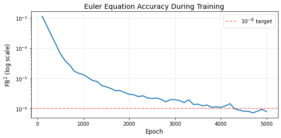
# === Plot 2: Learned Policy Functions ===
fig, axes = plt.subplots(1, 2, figsize=(13, 5))
colors = ["#1f77b4", "#ff7f0e"]
labels_eps = [r"$\varepsilon_L$ (low income)", r"$\varepsilon_H$ (high income)"]
labels_Z = ["$Z_L$ (recession)", "$Z_H$ (boom)"]

# Mean K from buffer distributions
buf_K = float(np.mean([
    np.sum(np.asarray(m) * np.asarray(k_grid)[None, :]) for m in buffer_mu
]))

for z_idx in range(N_Z):
    z_hist = jnp.full(H, z_idx, dtype=jnp.int32)
    agg_input = encode_Z_history(z_hist)
    R, w = compute_prices(max(buf_K, 0.01), 1.0, float(Z_VALS[z_idx]))
    c_grid_learned = np.asarray(actor_c_grid(psi, agg_input, float(R), float(w)))

    ls = '-' if z_idx == 0 else '--'
    for e in range(N_EPS):
        m = float(w) * float(EPS_VALS[e]) + float(R) * k_np
        axes[0].plot(k_np, c_grid_learned[e], color=colors[e], linestyle=ls,
                     linewidth=2, label=f"{labels_eps[e]}, {labels_Z[z_idx]}")

        # MPC at k=0: consumption as fraction of cash-on-hand (= boundary MPC α)
        mpc = np.zeros_like(k_np)
        mpc[0] = c_grid_learned[e, 0] / max(m[0], 1e-10)
        # MPC at k>0: finite-difference Δc/Δm = Δc/(R·Δk), matches I-spline MPC by construction
        mpc[1:] = np.diff(c_grid_learned[e]) / (float(R) * np.asarray(dk))
        axes[1].plot(k_np, mpc, color=colors[e], linestyle=ls, linewidth=2)

axes[0].set_xlabel("Capital $k$", fontsize=12)
axes[0].set_ylabel("Consumption $c$", fontsize=12)
axes[0].set_title("Learned consumption policy", fontsize=14)
axes[0].legend(fontsize=8, loc='lower right')
axes[0].grid(True, alpha=0.3)
axes[0].set_xlim(0, min(50, K_MAX))

axes[1].set_xlabel("Capital $k$", fontsize=12)
axes[1].set_ylabel("MPC", fontsize=12)
axes[1].set_title("Marginal propensity to consume", fontsize=14)
axes[1].set_ylim(-0.05, 1.05)
axes[1].grid(True, alpha=0.3)
axes[1].set_xlim(0, min(50, K_MAX))

plt.tight_layout()
plt.show()

# shape_report (defined in the initial-visualization cell above) verifies
# the four I-spline guarantees: c increasing, feasible, MPC ∈ [0,1], MPC decreasing
shape_report(c_grid_learned, float(R), float(w), "trained policy in the final plotted state")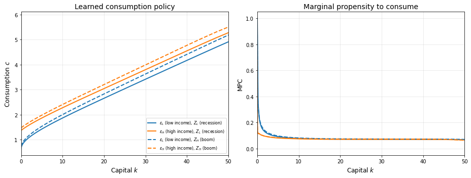
Shape check for trained policy in the final plotted state:
  min Δc across grid intervals      =  5.641e-03  (should be >= 0)
  max(c - cash on hand)             = -5.247e-04  (should be <= 0)
  MPC range on intervals            = [ 0.009,  0.633]
  max increase in MPC across k-grid = -3.123e-05  (should be <= 0)
Part 7: Euler Error Diagnostics¶
A single FB² number tells us the average accuracy, but not where the policy is good or bad. To diagnose this, we evaluate the per-grid-point Euler gap and Fischer-Burmeister residual across all replay buffer states.
Two diagnostic plots:
Consumption and MPC vs : how does the policy respond to different aggregate capital levels? (Approximate aggregation predicts these should be tight clouds.)
Euler / FB error bands: median and 10th–90th percentile bands of across the individual capital grid, separately for each income state .
# === Euler Error Diagnostics ===

def euler_diagnostics_one_state(psi, z_history, mu):
    """Per-grid-point Euler gap (g) and FB residual for one buffer state.

    Same computation as fb_loss_one_state but returns the full (eps, k) grids
    instead of a scalar mean, plus the consumption and MPC schedules.
    """
    z_t = z_history[-1]

    K_t, L_t = distribution_aggregates(mu)
    R_t, w_t = compute_prices(float(K_t), float(L_t), Z_VALS[z_t])
    R_t_f, w_t_f = float(R_t), float(w_t)

    agg_input = encode_Z_history(z_history)
    c_grid_t = actor_c_grid(psi, agg_input, R_t_f, w_t_f)

    m_grid = w_t_f * EPS_VALS[:, None] + R_t_f * k_grid[None, :]
    k_next_grid = jnp.clip(m_grid - c_grid_t, 0.0, k_grid[-1])

    # Next-period aggregates from Young step
    mu_next = distribution_step(mu, c_grid_t, R_t_f, w_t_f)
    K_next, L_next = distribution_aggregates(mu_next)
    K_next_f, L_next_f = float(K_next), float(L_next)

    q = jnp.zeros_like(c_grid_t)
    for z_next in range(N_Z):
        z_hist_next = jnp.concatenate([z_history[1:], jnp.array([z_next])])
        agg_next = encode_Z_history(z_hist_next)
        R_next, w_next = compute_prices(K_next_f, L_next_f, Z_VALS[z_next])
        R_nf, w_nf = float(R_next), float(w_next)
        c_grid_next = actor_c_grid(psi, agg_next, R_nf, w_nf)

        def _interp_next(i_next):
            k_flat = k_next_grid.ravel()
            idx = jnp.full(k_flat.shape, i_next, dtype=jnp.int32)
            return interpolate(c_grid_next, idx, k_flat).reshape(N_EPS, N + 1)

        c_next_all = jax.vmap(_interp_next)(jnp.arange(N_EPS))
        mu_u = 1.0 / jnp.maximum(c_next_all, 1e-10)
        exp_uc = jnp.einsum('ij,jik->ik', PI_EPS, mu_u)
        q += PI_Z[z_t, z_next] * BETA * R_nf * exp_uc

    c_euler = 1.0 / jnp.maximum(q, 1e-10)
    c_scale = jnp.maximum(c_grid_t, 1e-10)
    g_grid = (c_euler - c_grid_t) / c_scale
    s_grid = k_next_grid / c_scale
    fb_grid = jnp.sqrt(g_grid**2 + s_grid**2 + 1e-12) - g_grid - s_grid

    # MPC via finite-difference (= I-spline MPC at grid points by construction)
    c_np = np.asarray(c_grid_t)
    m_np = np.asarray(m_grid)
    mpc = np.zeros_like(c_np)
    mpc[:, 0] = c_np[:, 0] / np.maximum(m_np[:, 0], 1e-10)
    mpc[:, 1:] = np.diff(c_np, axis=1) / (R_t_f * np.asarray(dk)[None, :])

    return {
        "K": float(K_t), "c_grid": c_np, "mpc_grid": mpc,
        "g_grid": np.asarray(g_grid), "fb_grid": np.asarray(fb_grid),
    }

# Evaluate on all buffer states
print(f"Running Euler diagnostics on {len(buffer_z)} buffer states...")
diag_results = []
for i in range(len(buffer_z)):
    d = euler_diagnostics_one_state(
        psi, jnp.array(buffer_z[i]), jnp.array(buffer_mu[i])
    )
    diag_results.append(d)

all_K = np.array([d["K"] for d in diag_results])
all_c = np.stack([d["c_grid"] for d in diag_results])        # (n_states, N_EPS, N+1)
all_mpc = np.stack([d["mpc_grid"] for d in diag_results])    # (n_states, N_EPS, N+1)
abs_g = np.abs(np.stack([d["g_grid"] for d in diag_results]))
abs_fb = np.abs(np.stack([d["fb_grid"] for d in diag_results]))

print(f"K range: [{all_K.min():.2f}, {all_K.max():.2f}]")
print(f"Mean |g| = {abs_g.mean():.2e},  Mean FB² = {(abs_fb**2).mean():.2e}")
Running Euler diagnostics on 128 buffer states...
K range: [7.43, 9.60]
Mean |g| = 1.04e-03,  Mean FB² = 8.58e-07
# === Scatter: Consumption and MPC vs Aggregate Capital K ===
# At selected individual capital levels, how do c and MPC vary with the
# aggregate state?  Tight scatter clouds = approximate aggregation holds.

target_k_vals = [0.0, 1.0, 3.0, 7.0, 15.0, 30.0, float(k_np[-1])]
target_k_vals = [tk for tk in target_k_vals if tk <= float(k_np[-1])]
k_indices = [int(np.argmin(np.abs(k_np - tk))) for tk in target_k_vals]

colors_eps = ["#1f77b4", "#ff7f0e"]
eps_labels = [r"$\varepsilon_L$", r"$\varepsilon_H$"]

fig, axes = plt.subplots(2, len(k_indices), figsize=(3.5 * len(k_indices), 8),
                         sharex=True)
for col, ki in enumerate(k_indices):
    for e in range(N_EPS):
        axes[0, col].scatter(all_K, all_c[:, e, ki], s=3, alpha=0.3,
                             color=colors_eps[e],
                             label=eps_labels[e] if col == 0 else None)
        axes[1, col].scatter(all_K, all_mpc[:, e, ki], s=3, alpha=0.3,
                             color=colors_eps[e])

    axes[0, col].set_title(f"$k = {k_np[ki]:.1f}$", fontsize=9)
    axes[1, col].set_xlabel("$K$", fontsize=9)
    axes[0, col].grid(True, alpha=0.3)
    axes[1, col].grid(True, alpha=0.3)
    axes[0, col].tick_params(labelsize=7)
    axes[1, col].tick_params(labelsize=7)

axes[0, 0].set_ylabel("Consumption $c$")
axes[1, 0].set_ylabel("MPC")
axes[0, 0].legend(fontsize=7, markerscale=3)
fig.suptitle("Consumption and MPC vs aggregate capital $K$", fontsize=13, y=1.02)
plt.tight_layout()
plt.show()

print("Each column is a fixed individual capital level k.")
print("Variation across K comes from the encoder mapping different Z-histories to different policy coefficients.")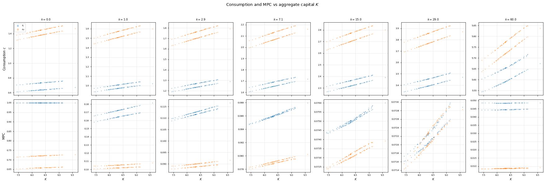
Each column is a fixed individual capital level k.
Variation across K comes from the encoder mapping different Z-histories to different policy coefficients.
# === Euler / FB Error Bands ===
# Median (line) and 10th–90th percentile (band) of |g| and |FB(g,s)|
# across replay buffer states, for each income state.

n_states = abs_g.shape[0]
fig, axes = plt.subplots(1, N_EPS, figsize=(6.2 * N_EPS, 8.2), sharex=True)

for i in range(N_EPS):
    fb_med = np.median(abs_fb[:, i, :], axis=0)
    fb_p10 = np.percentile(abs_fb[:, i, :], 10.0, axis=0)
    fb_p90 = np.percentile(abs_fb[:, i, :], 90.0, axis=0)

    # |FB| panel
    axes[i].fill_between(k_np, np.maximum(fb_p10, 1e-12),
                            np.maximum(fb_p90, 1e-12),
                            color=colors_eps[i], alpha=0.18)
    axes[i].plot(k_np, np.maximum(fb_med, 1e-12),
                    color=colors_eps[i], linewidth=2.0)
    axes[i].set_yscale("log")
    axes[i].set_ylabel(r"$|FB(g,s)|$")
    axes[i].set_xlabel("Capital $k$")
    axes[i].grid(True, alpha=0.3)


fig.suptitle(
    f"Replay-state one-step Euler / FB diagnostic ({n_states} states)",
    fontsize=13, y=1.02)
plt.tight_layout()
plt.show()

print("The band shows the 10th–90th percentile range across buffer states.")
print("Wider bands indicate more variation in accuracy across aggregate states.")
print("High |g| near k=0 reflects the borrowing constraint; high |g| at high k")
print("is often on grid points with zero household mass.")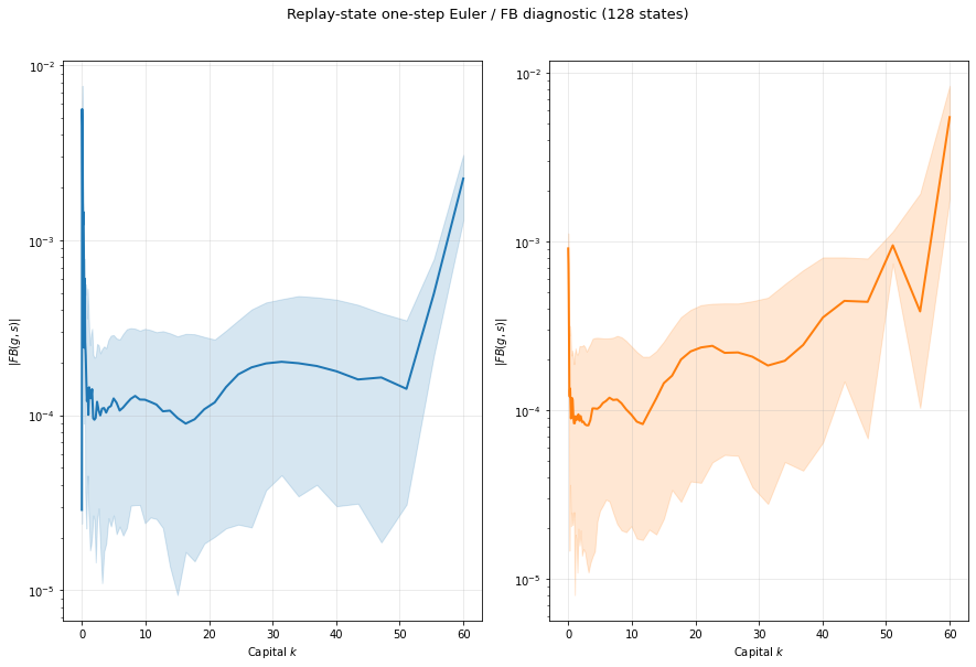
The band shows the 10th–90th percentile range across buffer states.
Wider bands indicate more variation in accuracy across aggregate states.
High |g| near k=0 reflects the borrowing constraint; high |g| at high k
is often on grid points with zero household mass.
Summary¶
In this notebook we:
Represented the consumption policy with an I-spline MPC basis, so the grid policy is increasing, concave, and feasible by construction.
Evaluated equilibrium conditions with a Fischer-Burmeister residual that handles both interior and constrained households.
Trained on a replay buffer of aggregate histories and household distributions.
Diagnosed solution quality with per-grid-point Euler error bands and scatter plots showing how the policy varies with the aggregate state.
Takeaways
The I-spline MPC representation gives a concrete example of how economic shape restrictions can be built directly into a neural network.
The replay buffer is the bridge between individual policies and aggregate prices.
The scatter plot of consumption vs at fixed visualizes approximate aggregation — tight clouds mean the policy depends mainly on prices, not on the full distribution.
The Euler/FB error band plot reveals where accuracy is best (interior ) and worst (near constraints and at high with zero household mass).
A few intentional simplifications
two-state aggregate and idiosyncratic Markov chains,
log utility,
a deterministic used only as a benchmark line.
Once this notebook feels comfortable, the GPU version shows how to move the same logic into a fully JIT-compiled training loop (still working on it).