Lecture 11, Notebook 05: The Black-Scholes PDE with a PINN - Deep Learning for Solving and Estimating Dynamic Models in Economics and Finance

Course: Deep Learning for Solving and Estimating Dynamic Models in Economics and Finance
Script reference: §7.8 (the Black-Scholes PDE)
Notebook role: core
Author: Simon Scheidegger

Run mode. The checked-in run uses RUN_MODE = "smoke" for fast execution; the accuracy figures quoted in the slides and the companion script use the longer teaching / production budgets. Set RUN_MODE in the next cell accordingly to reproduce them.

RUN_MODE = "smoke"  # one of: "smoke", "teaching", "production"
SEED = 0

Solving the Black-Scholes PDE with Physics-Informed Neural Networks¶

This notebook demonstrates how to solve the Black-Scholes partial differential equation for European call option pricing using a Physics-Informed Neural Network (PINN).

Relevance to Central Banking¶

Option pricing models are a cornerstone of modern financial risk management. Central banks routinely monitor option-implied measures — such as implied volatilities, risk-neutral densities, and the Greeks — to assess market expectations and gauge financial stability. The Black-Scholes model, while stylized, provides the canonical framework on which more realistic models are built.

PINNs offer a mesh-free, differentiable alternative to traditional finite-difference solvers for pricing PDEs. Because PINNs leverage automatic differentiation, they yield the option price and its sensitivities (the Greeks) simultaneously, without any additional numerical effort. This makes them attractive for stress-testing and scenario analysis in supervisory contexts.

The Black-Scholes PDE¶

For a European call option with value $V(S,t)$ , the PDE reads:

\frac{\partial V}{\partial t} + \frac{1}{2}\sigma^2 S^2 \frac{\partial^2 V}{\partial S^2} + r S \frac{\partial V}{\partial S} - r V = 0,

(1)

subject to:

Terminal condition: $V(S, T) = \max(S - K, 0)$
Boundary at $S=0$ : $V(0, t) = 0$
Boundary at $S=S_{\max}$ : $V(S_{\max}, t) = S_{\max} - K e^{-r(T-t)}$

Self-study notebook \u2014 This notebook complements the in-class PINNs session (Day 6, Block 1). Work through it at your own pace.


import torch
import torch.nn as nn
import torch.optim as optim
import numpy as np
import matplotlib.pyplot as plt
from scipy.stats import norm

plt.rcParams['font.size'] = 13

# Reproducibility
np.random.seed(SEED)
torch.manual_seed(SEED)
torch.set_default_dtype(torch.float64)

# torch.compile is not used in this notebook. The residual contains nested
# autograd calls, and the deterministic L-BFGS polish is easier to inspect in
# plain eager mode.


# ── Device setup ──────────────────────────────────────────────────────
device = torch.device("cuda" if torch.cuda.is_available() else "cpu")
dtype = torch.float64
print(f"Using device: {device} | dtype: {dtype}")

# ── Black-Scholes parameters ─────────────────────────────────────────
r     = 0.05    # risk-free rate
sigma = 0.2     # volatility
K     = 50.0    # strike price
T     = 1.0     # maturity (years)
S_max = 100.0   # upper bound on spot price domain

Using device: cpu | dtype: torch.float64

# Run-mode budget: hyperparameters dispatched from RUN_MODE (set in the second cell).
#   smoke      -- CPU-bounded smoke run for CI
#   teaching   -- laptop-scale figures
#   production -- full reproduction
_RUN_HP = {
    "smoke":      {"adam_lr": 1e-3, "n_epochs":  500, "n_interior":  300, "n_bc":  64, "n_terminal": 128, "n_bc_Smax":  64, "terminal_weight": 10.0, "lbfgs_iters":  80, "lbfgs_design": [ 512, 128,  256, 128], "adam_print_every":  100, "milestones": [240, 400],   "gamma_lr": 0.4},
    "teaching":   {"adam_lr": 1e-3, "n_epochs": 2500, "n_interior": 1000, "n_bc": 256, "n_terminal": 512, "n_bc_Smax": 256, "terminal_weight": 10.0, "lbfgs_iters": 300, "lbfgs_design": [2048, 512, 1024, 512], "adam_print_every":  500, "milestones": [1200, 2000], "gamma_lr": 0.4},
    "production": {"adam_lr": 1e-3, "n_epochs": 8000, "n_interior": 2000, "n_bc": 512, "n_terminal": 1024, "n_bc_Smax": 512, "terminal_weight": 10.0, "lbfgs_iters": 600, "lbfgs_design": [4096, 1024, 2048, 1024], "adam_print_every": 1000, "milestones": [4000, 6500], "gamma_lr": 0.4},
}
if RUN_MODE not in _RUN_HP:
    raise ValueError(f"RUN_MODE must be one of {list(_RUN_HP)}")
HP = _RUN_HP[RUN_MODE]
print(f"RUN_MODE={RUN_MODE!r}; SEED={SEED}; hyperparameters: {HP}")

RUN_MODE='smoke'; SEED=0; hyperparameters: {'adam_lr': 0.001, 'n_epochs': 500, 'n_interior': 300, 'n_bc': 64, 'n_terminal': 128, 'n_bc_Smax': 64, 'terminal_weight': 10.0, 'lbfgs_iters': 80, 'lbfgs_design': [512, 128, 256, 128], 'adam_print_every': 100, 'milestones': [240, 400], 'gamma_lr': 0.4}

PINN Architecture¶

The network takes a two-dimensional input $(S, t)$ and outputs the option value $V(S, t)$ . We use a fully connected feed-forward network with three hidden layers of 50 neurons each and $\tanh$ activation functions (smooth activations are important because the PDE loss requires second-order derivatives).


class PINN(nn.Module):
    """Physics-Informed Neural Network for the Black-Scholes PDE.

    Inputs are normalised to [-1, 1] and the output is scaled by the strike.
    This makes the PDE, terminal, and boundary losses numerically comparable.
    """

    def __init__(self, layer_sizes=None, S_max=S_max, T=T, price_scale=K):
        super().__init__()
        if layer_sizes is None:
            layer_sizes = [2, 64, 64, 64, 1]
        self.S_max = float(S_max)
        self.T = float(T)
        self.price_scale = float(price_scale)

        layers = []
        for i in range(len(layer_sizes) - 2):
            layers += [nn.Linear(layer_sizes[i], layer_sizes[i + 1]), nn.Tanh()]
        layers += [nn.Linear(layer_sizes[-2], layer_sizes[-1])]
        self.net = nn.Sequential(*layers)

    def forward(self, S, t):
        S_n = 2.0 * S / self.S_max - 1.0
        t_n = 2.0 * t / self.T - 1.0
        return self.price_scale * self.net(torch.cat([S_n, t_n], dim=1))


model = PINN().to(device=device, dtype=dtype)
print(model)

PINN(
  (net): Sequential(
    (0): Linear(in_features=2, out_features=64, bias=True)
    (1): Tanh()
    (2): Linear(in_features=64, out_features=64, bias=True)
    (3): Tanh()
    (4): Linear(in_features=64, out_features=64, bias=True)
    (5): Tanh()
    (6): Linear(in_features=64, out_features=1, bias=True)
  )
)

PDE Residual via Automatic Differentiation¶

The key idea behind PINNs is to enforce the PDE in its strong form at a set of collocation points. We compute the required partial derivatives $V_t$ , $V_S$ , and $V_{SS}$ using PyTorch’s automatic differentiation engine (torch.autograd.grad). The PDE residual should be driven to zero during training.


def pde_residual(model, S, t):
    """
    Compute the Black-Scholes PDE residual:
        R = V_t + 0.5*sigma^2*S^2*V_SS + r*S*V_S - r*V
    """
    S = S.clone().detach().requires_grad_(True)
    t = t.clone().detach().requires_grad_(True)

    V = model(S, t)
    V_t = torch.autograd.grad(
        V, t, grad_outputs=torch.ones_like(V),
        create_graph=True, retain_graph=True
    )[0]
    V_S = torch.autograd.grad(
        V, S, grad_outputs=torch.ones_like(V),
        create_graph=True, retain_graph=True
    )[0]
    V_SS = torch.autograd.grad(
        V_S, S, grad_outputs=torch.ones_like(V_S),
        create_graph=True, retain_graph=True
    )[0]

    residual = V_t + 0.5 * sigma**2 * S**2 * V_SS + r * S * V_S - r * V
    return residual

Sampling Collocation Points¶

We draw random collocation points in the interior of the domain $[0, S_{\max}] \times [0, T]$ as well as on each boundary (the terminal condition, the $S=0$ boundary, and the $S=S_{\max}$ boundary). Points are resampled every epoch so the network does not overfit to a fixed grid.


def sampler(n_interior, n_bc, n_terminal, n_bc_Smax):
    """Sample collocation, boundary, and terminal points."""
    S_int = torch.rand(n_interior, 1, device=device, dtype=dtype) * S_max
    t_int = torch.rand(n_interior, 1, device=device, dtype=dtype) * T

    S_bc0 = torch.zeros(n_bc, 1, device=device, dtype=dtype)
    t_bc0 = torch.rand(n_bc, 1, device=device, dtype=dtype) * T

    S_term = torch.rand(n_terminal, 1, device=device, dtype=dtype) * S_max
    t_term = torch.ones(n_terminal, 1, device=device, dtype=dtype) * T

    S_bcmax = torch.ones(n_bc_Smax, 1, device=device, dtype=dtype) * S_max
    t_bcmax = torch.rand(n_bc_Smax, 1, device=device, dtype=dtype) * T

    return (S_int, t_int, S_bc0, t_bc0, S_term, t_term, S_bcmax, t_bcmax)

Training the PINN¶

The loss terms are divided by the strike so that a boundary error of one currency unit does not overwhelm the scaled PDE residual. We use Adam to reach the right basin and then run L-BFGS on a fixed double-precision training batch. This is the stage where double precision is especially useful, because L-BFGS line-search and stopping criteria are sensitive to small loss changes.


# Hyperparameters dispatched from RUN_MODE
adam_lr         = HP["adam_lr"]
n_epochs        = HP["n_epochs"]
n_interior      = HP["n_interior"]
n_bc            = HP["n_bc"]
n_terminal      = HP["n_terminal"]
n_bc_Smax       = HP["n_bc_Smax"]
terminal_weight = HP["terminal_weight"]

optimizer = optim.Adam(model.parameters(), lr=adam_lr)
scheduler = optim.lr_scheduler.MultiStepLR(optimizer, milestones=HP["milestones"], gamma=HP["gamma_lr"])
loss_history = []


def loss_terms(batch):
    S_int_, t_int_, S_bc0_, t_bc0_, S_term_, t_term_, S_bcmax_, t_bcmax_ = batch

    res = pde_residual(model, S_int_, t_int_) / K
    mse_pde = torch.mean(res ** 2)

    V_bc0 = model(S_bc0_, t_bc0_) / K
    mse_bc0 = torch.mean(V_bc0 ** 2)

    V_term = model(S_term_, t_term_) / K
    payoff = torch.relu(S_term_ - K) / K
    mse_terminal = torch.mean((V_term - payoff) ** 2)

    V_bcmax = model(S_bcmax_, t_bcmax_) / K
    V_bcmax_exact = (S_max - K * torch.exp(-r * (T - t_bcmax_))) / K
    mse_bcmax = torch.mean((V_bcmax - V_bcmax_exact) ** 2)

    loss = mse_pde + mse_bc0 + terminal_weight * mse_terminal + mse_bcmax
    return loss, mse_pde, mse_bc0, mse_terminal, mse_bcmax


for epoch in range(1, n_epochs + 1):
    batch = sampler(n_interior, n_bc, n_terminal, n_bc_Smax)
    optimizer.zero_grad()
    loss, mse_pde, mse_bc0, mse_terminal, mse_bcmax = loss_terms(batch)
    loss.backward()
    torch.nn.utils.clip_grad_norm_(model.parameters(), 50.0)
    optimizer.step()
    scheduler.step()
    loss_history.append(loss.item())

    if epoch % HP["adam_print_every"] == 0 or epoch == 1:
        print(
            f"Adam {epoch:>5d}/{n_epochs}  "
            f"Loss: {loss.item():.4e}  "
            f"(PDE: {mse_pde.item():.3e}, "
            f"BC0: {mse_bc0.item():.3e}, "
            f"Term: {mse_terminal.item():.3e}, "
            f"BCmax: {mse_bcmax.item():.3e})"
        )

# Deterministic FP64 L-BFGS polish on one fixed design.
lbfgs_batch = sampler(*HP["lbfgs_design"])
lbfgs = optim.LBFGS(
    model.parameters(),
    max_iter=HP["lbfgs_iters"],
    tolerance_grad=1e-12,
    tolerance_change=1e-14,
    line_search_fn="strong_wolfe",
)
lbfgs_evals = [0]


def lbfgs_closure():
    lbfgs.zero_grad()
    loss, mse_pde, mse_bc0, mse_terminal, mse_bcmax = loss_terms(lbfgs_batch)
    loss.backward()
    lbfgs_evals[0] += 1
    if lbfgs_evals[0] == 1 or lbfgs_evals[0] % 50 == 0:
        print(
            f"L-BFGS eval {lbfgs_evals[0]:>4d} | loss={loss.item():.3e} "
            f"(pde={mse_pde.item():.1e}, term={mse_terminal.item():.1e})"
        )
    return loss

lbfgs.step(lbfgs_closure)
print(f"Final deterministic training loss: {lbfgs_closure().item():.3e}")

Adam     1/500  Loss: 1.7991e+00  (PDE: 3.220e-02, BC0: 1.782e-02, Term: 1.143e-01, BCmax: 6.060e-01)

Adam   100/500  Loss: 1.1139e-01  (PDE: 1.538e-02, BC0: 1.256e-02, Term: 7.606e-03, BCmax: 7.380e-03)

Adam   200/500  Loss: 1.1336e-02  (PDE: 4.141e-03, BC0: 7.340e-04, Term: 5.346e-04, BCmax: 1.115e-03)

Adam   300/500  Loss: 9.1765e-03  (PDE: 3.367e-03, BC0: 5.253e-04, Term: 4.529e-04, BCmax: 7.545e-04)

Adam   400/500  Loss: 8.0466e-03  (PDE: 3.296e-03, BC0: 5.101e-04, Term: 3.705e-04, BCmax: 5.356e-04)

Adam   500/500  Loss: 7.6889e-03  (PDE: 2.591e-03, BC0: 5.702e-04, Term: 3.952e-04, BCmax: 5.757e-04)
L-BFGS eval    1 | loss=7.751e-03 (pde=2.9e-03, term=3.8e-04)

L-BFGS eval   50 | loss=1.109e-03 (pde=3.1e-04, term=7.7e-05)

Final deterministic training loss: 5.310e-04

Analytical Black-Scholes Formula¶

For validation we compare the PINN solution against the closed-form Black-Scholes formula for a European call:

C(S, t) = S\,\Phi(d_1) - K e^{-r(T-t)}\Phi(d_2),

(2)

where $d_1 = \frac{\ln(S/K) + (r + \sigma^2/2)(T-t)}{\sigma\sqrt{T-t}}$ and $d_2 = d_1 - \sigma\sqrt{T-t}$ .

def black_scholes_call(S, K, T_minus_t, r, sigma):
    """
    Analytical Black-Scholes price for a European call.

    Parameters
    ----------
    S          : array-like, spot price
    K          : float, strike
    T_minus_t  : float, time to maturity
    r          : float, risk-free rate
    sigma      : float, volatility

    Returns
    -------
    C : np.ndarray, call prices
    """
    S = np.asarray(S, dtype=np.float64)
    # Handle S = 0 gracefully
    C = np.zeros_like(S)
    mask = S > 0
    d1 = (np.log(S[mask] / K) + (r + 0.5 * sigma**2) * T_minus_t) / (
        sigma * np.sqrt(T_minus_t)
    )
    d2 = d1 - sigma * np.sqrt(T_minus_t)
    C[mask] = S[mask] * norm.cdf(d1) - K * np.exp(-r * T_minus_t) * norm.cdf(d2)
    return C

Comparison: PINN vs. Analytical Solution¶

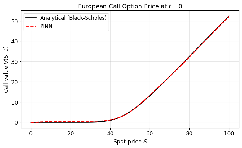
We evaluate both the trained PINN and the analytical formula at $t = 0$ (i.e. time to maturity $= T$ ) across the full range of spot prices.


# Evaluate at t = 0
S_test_np = np.linspace(0, S_max, 200)
S_test = torch.tensor(S_test_np, dtype=dtype, device=device).reshape(-1, 1)
t_test = torch.zeros_like(S_test)

model.eval()
with torch.no_grad():
    V_pinn = model(S_test, t_test).cpu().numpy().flatten()

V_exact = black_scholes_call(S_test_np, K, T, r, sigma)

# ── Plot ──────────────────────────────────────────────────────────────
fig, ax = plt.subplots(figsize=(8, 5))
ax.plot(S_test_np, V_exact, "k-", linewidth=2, label="Analytical (Black-Scholes)")
ax.plot(S_test_np, V_pinn, "r--", linewidth=2, label="PINN")
ax.set_xlabel(r"Spot price $S$", fontsize=13)
ax.set_ylabel("Call value $V(S, 0)$", fontsize=13)
ax.set_title(r"European Call Option Price at $t = 0$", fontsize=14)
ax.legend(fontsize=12)
ax.grid(True, alpha=0.3)
plt.tight_layout()
plt.show()

Error Analysis¶

We quantify the point-wise absolute error $|V_{\text{PINN}}(S,0) - V_{\text{exact}}(S,0)|$ across the spot-price domain.

abs_error = np.abs(V_pinn - V_exact)

fig, ax = plt.subplots(figsize=(8, 4))
ax.plot(S_test_np, abs_error, "b-", linewidth=1.5)
ax.set_xlabel(r"Spot price $S$", fontsize=13)
ax.set_ylabel("Absolute error", fontsize=13)
ax.set_title(r"Absolute Error: PINN vs. Analytical at $t = 0$", fontsize=14)
ax.grid(True, alpha=0.3)
plt.tight_layout()
plt.show()

print(f"Max  absolute error: {np.max(abs_error):.6f}")
print(f"Mean absolute error: {np.mean(abs_error):.6f}")

# ----- Final-error assertion (mode-dependent: max abs error vs Black-Scholes) -----
_tol = {"smoke": float("inf"), "teaching": 5e-1, "production": 1e-1}[RUN_MODE]
_max_err = float(np.max(abs_error))
assert _max_err < _tol, f"BS PINN max-abs-error {_max_err:.3e} exceeds tol {_tol:.0e} for RUN_MODE={RUN_MODE!r}"
print(f"\u2713 max-abs-error {_max_err:.3e} < {_tol:.0e}")

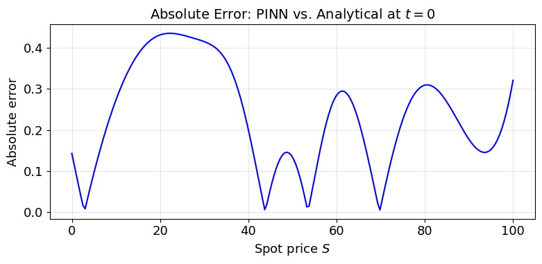
Max  absolute error: 0.435757
Mean absolute error: 0.235371
✓ max-abs-error 4.358e-01 < inf

Discussion: The Greeks¶

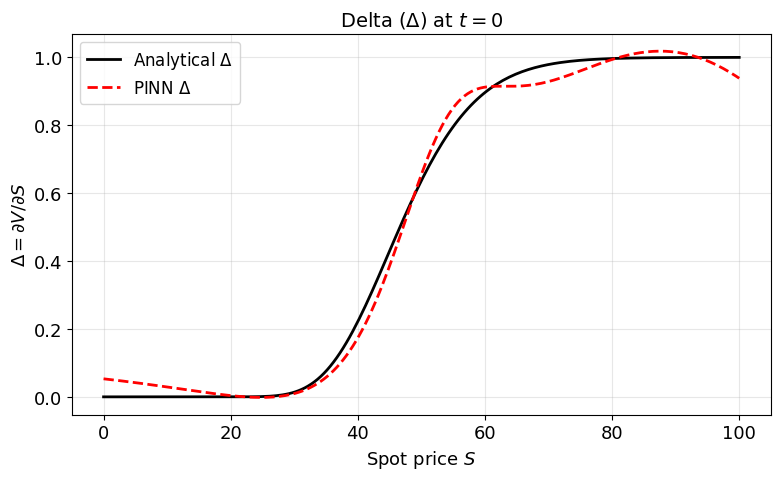
A powerful advantage of the PINN approach is that the Greeks — the price sensitivities with respect to the underlying parameters — are available essentially for free via automatic differentiation:

Greek	Definition	Interpretation
Delta	$\Delta = V_S$	Sensitivity to spot price
Gamma	$\Gamma = V_{SS}$	Convexity with respect to spot price
Theta	$\Theta = V_t$	Sensitivity to passage of time

There is no need for finite-difference bumping or re-solving the PDE. Below we illustrate this by computing Delta at $t = 0$ .


# Compute Delta = dV/dS at t = 0 via automatic differentiation
S_greek = torch.tensor(
    S_test_np, dtype=dtype, device=device
).reshape(-1, 1).requires_grad_(True)
t_greek = torch.zeros_like(S_greek)

V_greek = model(S_greek, t_greek)

delta = torch.autograd.grad(
    V_greek, S_greek,
    grad_outputs=torch.ones_like(V_greek),
    create_graph=False
)[0]

delta_np = delta.detach().cpu().numpy().flatten()

# Analytical Delta for comparison
mask = S_test_np > 0
delta_exact = np.zeros_like(S_test_np)
d1 = (np.log(S_test_np[mask] / K) + (r + 0.5 * sigma**2) * T) / (
    sigma * np.sqrt(T)
)
delta_exact[mask] = norm.cdf(d1)

# ── Plot ──────────────────────────────────────────────────────────────
fig, ax = plt.subplots(figsize=(8, 5))
ax.plot(S_test_np, delta_exact, "k-", linewidth=2, label=r"Analytical $\Delta$")
ax.plot(S_test_np, delta_np, "r--", linewidth=2, label=r"PINN $\Delta$")
ax.set_xlabel(r"Spot price $S$", fontsize=13)
ax.set_ylabel(r"$\Delta = \partial V / \partial S$", fontsize=13)
ax.set_title(r"Delta ($\Delta$) at $t = 0$", fontsize=14)
ax.legend(fontsize=12)
ax.grid(True, alpha=0.3)
plt.tight_layout()
plt.show()

Takeaway¶

The Black–Scholes PDE has a closed-form solution, so this notebook is a known-answer benchmark: we verify the PINN recipe (smooth activations, soft BCs with a tuned terminal weight, autodiff for V_S and V_SS, Adam-then-L-BFGS in FP64) before applying it to PDEs without closed forms (American options, jump diffusions, multi-asset pricing).
The Greeks (Δ = ∂V/∂S and beyond) come for free via torch.autograd.grad, one of the practical advantages of PINN-based pricing over many traditional numerical schemes that need separate finite-difference evaluations.
Quality of the fit at t = 0 should be checked against the analytical formula: if the PINN cannot recover Black–Scholes to plotting accuracy here, no further trust should be placed in its output on harder problems.