Course: Deep Learning for Solving and Estimating Dynamic Models in Economics and Finance
Script reference: §6.7 (Sequence-space DEQNs) -- Brock-Mirman warm-up
Notebook role: core
Author: Simon Scheidegger
# Run-mode switch (smoke = CPU-bounded for CI, teaching = laptop figures, production = full reproduction).
RUN_MODE = "smoke"  # one of: "smoke", "teaching", "production"
SEED = 0
Sequence-Space DEQN: Brock–Mirman Warm-Up¶
Status: in-class walkthrough — Day 4, sequence-space slot. This notebook is the simplest setting in which the sequence-space idea (network input = recent history of exogenous shocks instead of current endogenous aggregate state) can be made visible. The companion notebook
06_SequenceSpace_KrusellSmith.ipynb(TF2 teaching) and the JAX referenceKrusellSmith_Tutorial_CPU.ipynbapply the same template to the heterogeneous-agent benchmark.
Learning goals¶
By the end of this notebook you will be able to:
State the sequence-space formulation of a recursive equilibrium and explain the ergodicity-and-truncation argument that makes the truncated history a valid input for the policy network.
Recognise the single conceptual change versus a state-space DEQN: the network’s input changes (a shock-history window replaces the current endogenous aggregate state); the loss, the equilibrium conditions, and the gradient step are unchanged.
Read the four ingredients of the sequence-space cloud method as implemented here: a savings-rate network with sigmoid output, a Gauss–Hermite quadrature for the conditional expectation, a forward simulator that rolls the shock history one step at a time, and a per-episode SGD update on the squared Euler residual.
Validate the trained policy against the Brock–Mirman closed form (available under , log utility), and read the diagnostics: loss curve, ergodic state cloud, and policy / Euler-error histograms.
What this notebook is not¶
It is not a heterogeneous-agent solver. There is one representative household and one aggregate state. Sequence space here is a teaching device, not a dimensionality reduction. The payoff appears in the HA notebooks.
It does not use shape-preserving I-spline outputs. The sigmoid-savings-rate parameterisation is enough for the BM warm-up; I-splines enter in
06_…KrusellSmith.The loss is the direct residual minimisation algorithm of Azinovic-Yang & Žemlička (2025). The alternative time iteration with EGM algorithm is not used here.
References¶
Azinovic-Yang, M., & Žemlička, J. (2025). Deep learning in the sequence space. arXiv:2509.13623. Companion JAX repository:
azinoma/DeepLearningInTheSequenceSpace.Brock, W. A., & Mirman, L. J. (1972). Optimal economic growth and uncertainty: the discounted case. Journal of Economic Theory 4(3), 479–513.
1. The Brock–Mirman model¶
A representative household maximises
subject to the resource constraint
with full depreciation and an exogenous AR(1) for log productivity
Key analytic fact (used as a benchmark)¶
With and the planner’s policy is closed-form:
We use this as a ground truth in the diagnostic plots (§14). The notebook also runs in regimes where the closed form does not apply — those skip the policy-comparison plot.
2. State-space vs sequence-space — the same equilibrium, two domains¶
The classical state-space representation of the recursive equilibrium reads:
| Equation | Domain | |
|---|---|---|
| Recursive policy | state | |
| Transition | known function | |
| Functional equation | enforced on the state space |
The sequence-space representation expresses the same equilibrium policy as a function of the history of exogenous shocks instead of the current endogenous state:
| Equation | Domain | |
|---|---|---|
| Sequence-space policy | shock history | |
| Iterated law of motion | derived from | |
| Functional equation | enforced on the shock-history space |
Same equilibrium, different domain of approximation. The two formulations describe the same set of equilibrium policies. They differ in what the network takes as input. State-space inputs may be high-dimensional once a distribution enters; sequence-space inputs live on a (potentially long but) purely exogenous domain.
3. Ergodicity and truncation — why a finite history is enough¶
For a large class of economies the equilibrium policy satisfies the ergodicity property
i.e. the influence of long-past shocks decays. Truncating the history after lags gives a truncated sequence-space solution
Brock–Mirman makes this concrete¶
Iterating the BM transition (with , log utility, ) gives
so the lag- shock enters with weight . With , the lag-25 weight is — truncating at leaves negligible error. This is the entire justification for using a length-25 shock-history window as the network input.
4. Algorithm sketch — direct residual minimisation with a cloud method¶
The training loop has three pieces. We will see each one in code below.
Initialisation. Sample initial state-history pairs . We initialise all of them at the deterministic steady state with empty histories.
Per-episode training (mini-batch SGD).
Draw a mini-batch of cloud entries.
Forward-pass the network to get a savings rate , then , , and the implied .
For each Gauss–Hermite quadrature node, build the next-period shock history and run the network again to get .
Compute the squared Euler residual; backprop and Adam step.
Cloud refresh. After every episode, draw fresh shocks for the entire cloud and roll one period forward (forward-simulator step, no gradients). The cloud now lives one period later — the ergodic distribution under the current policy emerges over many episodes.
The cloud-method sampling concentrates training data on the ergodic set: states the model actually visits under the policy being trained, rather than uniformly drawn states which may include economically irrelevant regions.
5. Imports and TF/GPU setup¶
We use TensorFlow 2 / Keras. All later cells assume the imports and the symbol
USE_GPU are in scope.
# -*- coding: utf-8 -*-
"""
NCG_Sequence_1_TensorFlow.py

TensorFlow/Keras implementation of the sequence-space algorithm from the paper
"Deep Learning in the Sequence Space" by Azinovic-Yang and Žemlička,
with real-time progress monitoring and bug fixes.
"""

# (1) Import Libraries and Setup
import tensorflow as tf
import numpy as np
import matplotlib.pyplot as plt
import time
import sys

print("TensorFlow Version:", tf.__version__)

# Ensure GPU is being used if available
USE_GPU = True
if USE_GPU:
    physical_devices = tf.config.list_physical_devices('GPU')
    if len(physical_devices) > 0:
        tf.config.experimental.set_memory_growth(physical_devices[0], True)
        print("Using GPU:", physical_devices[0].name)
    else:
        print("GPU not found, using CPU.")
else:
    print("Using CPU.")
2026-04-22 23:27:21.823263: E external/local_xla/xla/stream_executor/cuda/cuda_fft.cc:477] Unable to register cuFFT factory: Attempting to register factory for plugin cuFFT when one has already been registered
WARNING: All log messages before absl::InitializeLog() is called are written to STDERR
E0000 00:00:1776893241.841538   44264 cuda_dnn.cc:8310] Unable to register cuDNN factory: Attempting to register factory for plugin cuDNN when one has already been registered
E0000 00:00:1776893241.847072   44264 cuda_blas.cc:1418] Unable to register cuBLAS factory: Attempting to register factory for plugin cuBLAS when one has already been registered
2026-04-22 23:27:21.864683: I tensorflow/core/platform/cpu_feature_guard.cc:210] This TensorFlow binary is optimized to use available CPU instructions in performance-critical operations.
To enable the following instructions: AVX2 FMA, in other operations, rebuild TensorFlow with the appropriate compiler flags.
TensorFlow Version: 2.18.0
GPU not found, using CPU.
2026-04-22 23:27:24.710630: E external/local_xla/xla/stream_executor/cuda/cuda_driver.cc:152] failed call to cuInit: INTERNAL: CUDA error: Failed call to cuInit: UNKNOWN ERROR (303)
6. Calibration¶
| Symbol | Value | Comment |
|---|---|---|
| capital share | ||
| 0.97 | discount factor | |
| 1.0 | log utility (BM closed form available) | |
| 1.0 | full depreciation (BM closed form available) | |
| 0.98 | TFP persistence | |
| 0.01 | TFP innovation std |
The choice is what unlocks the closed-form benchmark . Change either to a non-unit value and the analytical comparison plots in §14 are simply skipped.
State and policy index conventions¶
The state vector is 5-wide here, not 2-wide: in addition to we
pre-compute in ExpandState so the loss
function can read them off directly without recomputing each time. The policy vector
is 3-wide: savings , consumption , marginal utility .
# (4) Calibrate parameters
_alpha = 1/3
_beta = 0.97
_gamma = 1.0
_delta = 1.0
_rho_z = 0.98
_sigma_z = 0.01
_sigma_z_erg = _sigma_z / np.sqrt(1 - _rho_z**2)

# Create a params tensor for use in TF functions
params_init = tf.constant([_alpha, _beta, _gamma, _delta, _rho_z, _sigma_z], dtype=tf.float32)

# Parameter indices
idx_par_alpha = 0
idx_par_beta = 1
idx_par_gamma = 2
idx_par_delta = 3
idx_par_rho_z = 4
idx_par_sigma_z = 5

# State and policy indices
idx_state_k = 0
idx_state_z = 1
idx_state_Z = 2
idx_state_y = 3
idx_state_mpk = 4
n_state = 5

idx_policy_s = 0
idx_policy_c = 1
idx_policy_mu = 2
7. Algorithm hyperparameters and Gauss–Hermite quadrature¶
| Symbol | Value | Role |
|---|---|---|
N_neur_sequence | 64 | width of each hidden layer |
gh_order | 8 | Gauss–Hermite quadrature nodes per (one-dim) shock |
n_cloud | size of the simulated cloud | |
n_minib | mini-batch size for SGD | |
n_history | 25 | length of the shock-history window |
lr_adam | 10-5 | Adam learning rate |
cloud_steps | total training episodes |
The Gauss–Hermite nodes and weights are rescaled so that they integrate against the standard-normal density: nodes are multiplied by , weights divided by , so that
# (5) Algorithm Hyperparameters
N_neur_sequence = 64
gh_order = 8
eps_safe = 1e-6
n_cloud = 2**12
n_minib = 2**8
n_history = 25
lr_adam = 1e-5
cloud_steps = 256 * 8

# Gauss-Hermite Quadrature nodes and weights
nodes, weights = np.polynomial.hermite.hermgauss(gh_order)
nodes = tf.constant(nodes * np.sqrt(2), dtype=tf.float32)[:, tf.newaxis]
weights = tf.constant(weights / np.sqrt(np.pi), dtype=tf.float32)[:, tf.newaxis]
8. Deterministic steady state and initial state¶
At (so ), the deterministic steady state solves
With this gives . We use this point as the initial condition for every track of the cloud at episode 0; the policy-driven simulator then disperses the cloud to its ergodic distribution.
# Initial state (steady state)
_z_ss = 0.0
_Z_ss = np.exp(_z_ss)
_k_ss = (_Z_ss * _alpha / (1/_beta + _delta - 1))**(1/(1 - _alpha))
_y_ss = _Z_ss * _k_ss**_alpha + (1 - _delta) * _k_ss
_mpk_ss = _alpha * _Z_ss * _k_ss**(_alpha - 1) + (1 - _delta)
init_state_np = np.array([_k_ss, _z_ss, _Z_ss, _y_ss, _mpk_ss])
init_state = tf.constant(init_state_np, dtype=tf.float32)
9. Economic primitives — utility and the BM analytic policy¶
The helper mksp (“make positive”) clips its argument away from zero by adding a
tiny eps_safe. This avoids c < 0 blowing up u'(c) = c^{-\gamma} during the
early, untrained iterations.
Marginal utility and its inverse¶
u_c(c, params)returns . The factor scales the optimisation problem so that the value function is on a similar scale to per-period utility (bounded, normalised problem). It does not affect the policy.u_c_i(u, params)is the inverse: given a marginal utility level it returns the consumption that produces it. Used in the Euler residual to convert into “implied consumption today”.
Brock–Mirman closed form¶
BrockMirman(x, params) returns the analytic savings
for the case . We evaluate this on the trained cloud at the end
to verify the network learned the right policy.
# (7) Structure of the economy (TensorFlow implementation)
def mksp(x):
  return tf.abs(x) + eps_safe

@tf.function
def u_c(c, params):
  gamma = params[idx_par_gamma]
  beta = params[idx_par_beta]
  return (1 - beta) * mksp(c)**(-gamma)

@tf.function
def u_c_i(u_c_val, params):
  gamma = params[idx_par_gamma]
  beta = params[idx_par_beta]
  return mksp(u_c_val / (1 - beta))**(-1/gamma)

# (7.10) Brock and Mirman (1972) analytic policy function (for comparison)
@tf.function
def BrockMirman(x, params):
  alpha = params[idx_par_alpha]
  beta = params[idx_par_beta]
  k = x[..., idx_state_k]
  z = x[..., idx_state_z]
  y = tf.exp(z) * k**alpha
  s = alpha * beta * y
  return s
10. ExpandState: precompute derived state quantities¶
Given the core state , this returns the expanded 5-wide state .
The reason for storing these explicitly: the Euler residual computation later needs at each quadrature node. Building it inside the loss and watching TensorFlow trace the same algebra repeatedly would be wasteful; precomputing keeps the loss function clean.
# (8) Expanded State Function
@tf.function
def ExpandState(x, params):
  alpha = params[idx_par_alpha]
  delta = params[idx_par_delta]
  k = x[..., 0]
  z = x[..., 1]
  Z = tf.exp(z)
  y = Z * mksp(k)**alpha + (1 - delta) * k
  mpk = alpha * Z * k**(alpha - 1) + (1 - delta)
  return tf.stack([k, z, Z, y, mpk], axis=-1)
11. The sequence-space network¶
The network architecture is intentionally minimal:
Input. A length-25 vector of past innovations . At episode 0 the cloud has all-zero histories; histories grow as the simulator runs.
Hidden layers. Three dense layers of width 64 with
geluactivation.Output. A single scalar passed through
sigmoid— interpreted as the savings rate . This is a hard constraint in the spirit of Day 4 nb 02: feasibility (, hence and ) is built into the architecture, never a loss term.
Why predict the savings rate instead of directly? Two reasons:
the savings rate is bounded and a smoother function of the state (much easier for the network to learn than the raw level , which has a wide range);
cumulating recovers exactly without an extra layer.
# (9.2) Sequence-space network (TensorFlow/Keras)
def Build_sequence(input_shape):
  return tf.keras.Sequential([
      tf.keras.layers.Input(shape=(input_shape,)),
      tf.keras.layers.Dense(N_neur_sequence, activation='gelu'),
      tf.keras.layers.Dense(N_neur_sequence, activation='gelu'),
      tf.keras.layers.Dense(N_neur_sequence, activation='gelu'),
      tf.keras.layers.Dense(1, activation='sigmoid') # Predicts saving rate
  ])

# Instantiate the model and optimizer
network_sequence = Build_sequence(n_history)
optimizer = tf.keras.optimizers.Adam(learning_rate=lr_adam)
12. From network output to a full policy¶
Policy_sequence(x, history, model, params) reads the precomputed from the
expanded state, runs the network on the shock history to get the savings rate
, and returns the 3-wide policy vector
The 3-D-input branch in the function (if len(history.shape) == 3) handles the
batched evaluation across Gauss–Hermite quadrature nodes inside the Euler-residual
computation: there, each batch entry has 8 next-period histories (one per quadrature
node), so the input tensor has shape [batch, 8, 25] and we reshape to [batch*8, 25]
to feed Keras, then reshape the output back.
# (10.2) Policy Function (Sequence-space version) - CORRECTED
@tf.function
def Policy_sequence(x, history, model, params):
    y = x[..., idx_state_y:idx_state_y+1]

    # Reshape 3D inputs for the model and reshape the output back.
    # Shape check uses static shape for tracing compatibility
    if len(history.shape) == 3:
        # This handles the case for the 'next period' calculation in E_sequence
        shape = tf.shape(history); batch_size, gh_order_dim, n_hist = shape[0], shape[1], shape[2]
        history_reshaped = tf.reshape(history, (batch_size * gh_order_dim, n_hist))
        sav_rate_flat = model(history_reshaped, training=True)
        sav_rate = tf.reshape(sav_rate_flat, (batch_size, gh_order_dim, 1)) + eps_safe
    else:
        # This handles the standard 2D case
        sav_rate = model(history, training=True) + eps_safe

    s = sav_rate * y
    c = (1.0 - sav_rate) * y
    mu = u_c(c, params)

    return tf.concat([s, c, mu], axis=-1)
13. The Euler residual in sequence space — the loss core¶
The household’s stochastic Euler equation (with full depreciation ) is
Writing and integrating the conditional expectation by Gauss–Hermite,
The residual we minimise is the relative-error form
i.e. implied consumption today / actual consumption today − 1. Squaring and averaging over the cloud gives the loss.
What the function E_sequence does, step by step¶
Read , , from the current state and policy (
Policy_sequence).Build the next-period shock for each of 8 quadrature nodes — broadcasted over the batch (shape becomes
[batch, 8, 1]).Build the next-period expanded state at every quadrature node by feeding through
ExpandState.Build the next-period shock history by prepending each quadrature node and dropping the oldest entry of the current history (shape:
[batch, 8, 25]).Re-run the network at every quadrature node to get (this is the “second forward pass” — analogous to the second
tape.gradientcall in nb 02–04).Form the GH-weighted expectation, invert via
u_c_i, divide by , subtract 1.
Note: the network is called twice in this function — once at and once at every . Both calls use the same network weights , and TensorFlow correctly backpropagates through both.
# (11.2) Error Function (Sequence-space version)
@tf.function
def E_sequence(x_batch, history_batch, model, params):
    beta = params[idx_par_beta]
    rho_z = params[idx_par_rho_z]
    sigma_z = params[idx_par_sigma_z]

    z = x_batch[:, tf.newaxis, idx_state_z] # Shape: [batch_size, 1]

    policy = Policy_sequence(x_batch, history_batch, model, params)
    s = policy[..., idx_policy_s:idx_policy_s+1] # Shape: [batch_size, 1]
    c = policy[..., idx_policy_c:idx_policy_c+1] # Shape: [batch_size, 1]

    # Transpose nodes for broadcasting and add a dimension at the end.
    z_next = rho_z * z + sigma_z * tf.transpose(nodes) # Broadcasts [256, 1] + [1, 8] -> [256, 8]
    z_next = z_next[..., tf.newaxis] # Shape -> [256, 8, 1]

    k_next = s[:, tf.newaxis, :] * tf.ones_like(z_next) # Broadcasts [256, 1, 1] * [256, 8, 1] -> [256, 8, 1]

    x_next_core = tf.concat([k_next, z_next], axis=-1) # Shape: [256, 8, 2]
    x_next_expanded = ExpandState(x_next_core, params) # Shape: [256, 8, 5]
    mpk_next = x_next_expanded[..., idx_state_mpk] # Shape: [256, 8]

    # Correctly construct the next period histories for the batch.
    batch_size = tf.shape(x_batch)[0]
    history_truncated_expanded = history_batch[:, tf.newaxis, :-1] # Shape: [256, 1, 24]
    nodes_expanded = nodes[tf.newaxis, :, :] # Shape: [1, 8, 1]

    history_tiled = tf.tile(history_truncated_expanded, [1, gh_order, 1]) # Shape: [256, 8, 24]
    nodes_tiled = tf.tile(nodes_expanded, [batch_size, 1, 1]) # Shape: [256, 8, 1]

    history_next = tf.concat([nodes_tiled, history_tiled], axis=2) # Shape: [256, 8, 25]

    policy_next = Policy_sequence(x_next_expanded, history_next, model, params)
    mu_next = policy_next[..., idx_policy_mu] # Shape: [256, 8]

    eul_kernel = tf.transpose(weights) * mu_next * mpk_next # Broadcasts [1, 8] * [256, 8] * [256, 8]
    eul_expect = tf.reduce_sum(eul_kernel, axis=1, keepdims=True) # Shape: [256, 1]

    err_eul = u_c_i(beta * eul_expect, params) / c - 1.0
    return tf.squeeze(err_eul)
14. Forward simulator: rolling the shock history one period¶
ForwardStep_sequence is not used inside the loss — it is the cloud-refresh step.
For each cloud entry it draws a single innovation (the
epsilon argument), computes:
,
(the savings rate already returned ),
new expanded state via
ExpandState,new history — prepend the fresh innovation, drop the oldest.
Because the function is decorated with @tf.function and receives only constants
from outside the graph, TensorFlow compiles it once and reuses the trace each
episode — fast.
# (13.2) Forward Step (Sequence-space)
@tf.function
def ForwardStep_sequence(x, history, epsilon, model, params):
    rho_z = params[idx_par_rho_z]
    sigma_z = params[idx_par_sigma_z]

    policy = Policy_sequence(x, history, model, params)
    s = policy[..., idx_policy_s]
    z = x[..., idx_state_z]

    z_next = rho_z * z + sigma_z * tf.squeeze(epsilon)
    x_next_core = tf.stack([s, z_next], axis=-1)
    x_next = ExpandState(x_next_core, params)

    epsilon_reshaped = tf.reshape(epsilon, [-1, 1])
    history_next = tf.concat([epsilon_reshaped, history[:, :-1]], axis=1)

    return x_next, history_next
15. The single SGD step¶
train_step wraps the loss in a tf.GradientTape, computes the gradient of the
mean squared Euler residual w.r.t.\ the network’s trainable variables, and applies
one Adam step. Standard pattern; nothing model-specific here.
# (12 & 14) Loss and Update Step
@tf.function
def train_step(x_batch, history_batch, model, params):
  with tf.GradientTape() as tape:
    err_eul = E_sequence(x_batch, history_batch, model, params)
    loss = tf.reduce_mean(err_eul**2)

  gradients = tape.gradient(loss, model.trainable_variables)
  optimizer.apply_gradients(zip(gradients, model.trainable_variables))
  return loss
16. The cloud-method training loop¶
CloudMethod_sequence is the outer loop. Each episode:
Build a
tf.data.Datasetfrom the current cloud(x_cloud, history_cloud), shuffle, batch into mini-batches of sizen_minib = 256.Iterate over mini-batches, accumulate per-episode loss.
Print progress every 20 episodes.
Draw fresh shocks for the entire cloud (one shock per cloud entry, via
tf.random.normal), and roll forward one period withForwardStep_sequence.
The cloud entries’ histories grow by one entry each episode, until they fill the length-25 window after 25 episodes. From episode 25 onwards every entry has a “warm” history.
Runtime note. With the defaults (
cloud_steps = 2048,n_cloud = 4096,n_minib = 256, GH order 8) the loop does SGD steps, each evaluating the network on 256 + inputs. CPU runtime is in the 20-40 minute range; GPU compresses it to a few minutes.
# (16 & 17) Main Training Loop
def CloudMethod_sequence(cloud_steps, model, params):
    x_cloud = tf.tile(tf.expand_dims(init_state, 0), [n_cloud, 1])
    history_cloud = tf.zeros((n_cloud, n_history), dtype=tf.float32)

    loss_history = []

    print("Starting training...")
    start_time = time.time()

    for episode in range(cloud_steps):
        dataset = tf.data.Dataset.from_tensor_slices((x_cloud, history_cloud))
        dataset = dataset.shuffle(n_cloud).batch(n_minib)

        episode_loss = 0.0
        num_batches = 0
        for x_batch, history_batch in dataset:
            loss_val = train_step(x_batch, history_batch, model, params)
            episode_loss += loss_val
            num_batches += 1

        avg_loss = episode_loss / num_batches
        loss_history.append(avg_loss)

        # Real-time progress update
        if (episode + 1) % 20 == 0 or episode == cloud_steps - 1:
            elapsed = time.time() - start_time
            sys.stdout.write(
                f"\rEpisode {episode + 1}/{cloud_steps} | "
                f"Loss (MSE): {avg_loss:.4e} | "
                f"Elapsed Time: {elapsed:.2f}s"
            )
            sys.stdout.flush()

        shocks = tf.random.normal(shape=(n_cloud, 1), dtype=tf.float32)
        x_cloud, history_cloud = ForwardStep_sequence(x_cloud, history_cloud, shocks, model, params)

    print("\nTraining finished.")
    return x_cloud, history_cloud, np.array(loss_history)
# Run the training
x_final_seq, history_final_seq, loss_field_avg_sequence = CloudMethod_sequence(
    cloud_steps, network_sequence, params_init
)
Starting training...
2026-04-22 23:29:19.386324: I tensorflow/core/framework/local_rendezvous.cc:405] Local rendezvous is aborting with status: OUT_OF_RANGE: End of sequence
2026-04-22 23:29:19.681948: I tensorflow/core/framework/local_rendezvous.cc:405] Local rendezvous is aborting with status: OUT_OF_RANGE: End of sequence
2026-04-22 23:29:19.904151: I tensorflow/core/framework/local_rendezvous.cc:405] Local rendezvous is aborting with status: OUT_OF_RANGE: End of sequence
2026-04-22 23:29:20.388308: I tensorflow/core/framework/local_rendezvous.cc:405] Local rendezvous is aborting with status: OUT_OF_RANGE: End of sequence
2026-04-22 23:29:21.262552: I tensorflow/core/framework/local_rendezvous.cc:405] Local rendezvous is aborting with status: OUT_OF_RANGE: End of sequence
Episode 20/2048 | Loss (MSE): 2.8178e-01 | Elapsed Time: 4.13s2026-04-22 23:29:22.906582: I tensorflow/core/framework/local_rendezvous.cc:405] Local rendezvous is aborting with status: OUT_OF_RANGE: End of sequence
Episode 60/2048 | Loss (MSE): 8.5000e-02 | Elapsed Time: 8.26s2026-04-22 23:29:26.231227: I tensorflow/core/framework/local_rendezvous.cc:405] Local rendezvous is aborting with status: OUT_OF_RANGE: End of sequence
Episode 120/2048 | Loss (MSE): 3.4365e-02 | Elapsed Time: 14.20s2026-04-22 23:29:32.537287: I tensorflow/core/framework/local_rendezvous.cc:405] Local rendezvous is aborting with status: OUT_OF_RANGE: End of sequence
Episode 240/2048 | Loss (MSE): 1.5503e-02 | Elapsed Time: 26.49s2026-04-22 23:29:45.769582: I tensorflow/core/framework/local_rendezvous.cc:405] Local rendezvous is aborting with status: OUT_OF_RANGE: End of sequence
Episode 500/2048 | Loss (MSE): 2.3200e-03 | Elapsed Time: 55.26s2026-04-22 23:30:14.190880: I tensorflow/core/framework/local_rendezvous.cc:405] Local rendezvous is aborting with status: OUT_OF_RANGE: End of sequence
Episode 1020/2048 | Loss (MSE): 1.6262e-04 | Elapsed Time: 114.44s2026-04-22 23:31:12.420761: I tensorflow/core/framework/local_rendezvous.cc:405] Local rendezvous is aborting with status: OUT_OF_RANGE: End of sequence
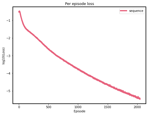
Episode 2048/2048 | Loss (MSE): 3.5160e-06 | Elapsed Time: 227.65s
Training finished.
2026-04-22 23:33:05.214055: I tensorflow/core/framework/local_rendezvous.cc:405] Local rendezvous is aborting with status: OUT_OF_RANGE: End of sequence
17. Diagnostics¶
Three diagnostic plots:
Loss curve ( of the per-episode mean squared Euler residual) — should decrease monotonically (with noise) and reach on the BM problem.
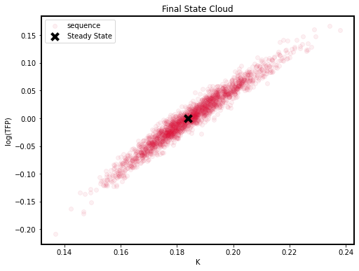
Final state cloud — the cloud should concentrate around the stochastic steady state, with spread set by the AR(1) dynamics.
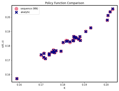
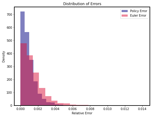
Policy comparison and error histograms — only shown when (closed-form available). The network’s savings should overlay the analytic ; the Euler-error histogram should sit at small relative error.
# --- Plotting and Analysis ---

# Plotting settings
plt.rcParams['font.size'] = 15
plt.rcParams['axes.linewidth'] = 2
plt.rcParams['lines.linewidth'] = 4
# 1. Per episode loss plot
plt.figure(figsize=(8, 6))
plt.plot(np.log10(loss_field_avg_sequence), color='crimson', alpha=2/3, label='sequence')
plt.legend()
plt.xlabel('Episode')
plt.ylabel('log10(Loss)')
plt.title('Per episode loss')
plt.show()
17.2 Ergodic state cloud¶
The scatter shows the final positions of all tracks at the end of training. We expect a tight blob around with spread along both axes set by the unconditional variance of the AR(1) productivity process.
# 2. State cloud scatter plot
plt.figure(figsize=(8, 6))
n_plot_batch = 2**11
plt.scatter(
    x_final_seq[:n_plot_batch, idx_state_k],
    x_final_seq[:n_plot_batch, idx_state_z],
    color='crimson', alpha=1/16, label='sequence'
)
plt.scatter(init_state_np[idx_state_k], init_state_np[idx_state_z], color='black', marker='x', s=100, label='Steady State')
plt.legend()
plt.xlabel('K')
plt.ylabel('log(TFP)')
plt.title('Final State Cloud')
plt.show()
17.3 Policy and Euler errors (only when )¶
If we are in the analytic regime, we overlay the network’s savings policy against on a few cloud samples, and plot the histogram of:
Policy error .
Euler error (relative form).
Both should be tightly concentrated at small values.
# 3. Policy and Euler error plot (if analytic solution available)
if _gamma == 1.0 and _delta == 1.0:
    y_analytic = BrockMirman(x_final_seq, params_init)
    policy_hat_sequence = Policy_sequence(x_final_seq, history_final_seq, network_sequence, params_init)
    y_hat_sequence = policy_hat_sequence[:, idx_policy_s]

    l1_sequence = tf.abs((y_analytic - y_hat_sequence) / y_analytic).numpy()
    eul_err = tf.abs(E_sequence(x_final_seq, history_final_seq, network_sequence, params_init)).numpy()

    # Policy scatter plot
    plt.figure(figsize=(8, 6))
    n_plot_policy_batch = 32
    plt.scatter(
        x_final_seq[:n_plot_policy_batch, idx_state_k],
        y_hat_sequence[:n_plot_policy_batch],
        color='crimson', alpha=0.5, label='sequence (NN)', marker='o', s=200
    )
    plt.scatter(
        x_final_seq[:n_plot_policy_batch, idx_state_k],
        y_analytic[:n_plot_policy_batch],
        color='navy', alpha=1.0, label='analytic', marker='x', s=100
    )
    plt.legend()
    plt.xlabel('K')
    plt.ylabel('s(K, z)')
    plt.title('Policy Function Comparison')
    plt.show()

    # Error histogram
    plt.figure(figsize=(8, 6))
    plt.hist(l1_sequence, bins=20, color='navy', alpha=0.5, label='Policy Error', density=True)
    plt.hist(eul_err, bins=20, color='crimson', alpha=0.5, label='Euler Error', density=True)
    plt.xlabel('Relative Error')
    plt.ylabel('Density')
    plt.title('Distribution of Errors')
    plt.legend()
    plt.show()
else:
    print("Analytic solution only available for gamma=1 and delta=1. Skipping policy comparison plots.")
18. Take-away¶
The single conceptual change versus the state-space DEQNs of Day 4 nb 02–03:
| Day 4 nb 02 (state-space) | This notebook (sequence-space) |
|---|---|
| Network input: current state — 2 floats. | Network input: shock history — 25 floats. |
| Network output: savings rate (or ). | Network output: savings rate. |
| Loss: squared Euler residual. | Loss: squared Euler residual. (unchanged) |
| Sampling: cloud method. | Sampling: cloud method. (unchanged) |
In the BM model the input swap is larger, not smaller — sequence space is a
teaching device here, not a dimensionality reduction. The motivation only pays off
in the heterogeneous-agent setting (06_SequenceSpace_KrusellSmith.ipynb and
KrusellSmith_Tutorial_CPU.ipynb), where the alternative input would be a 100-bin
histogram of agents’ wealth. There the shock history is genuinely smaller and
exogenous (does not move with the policy update) — which is the source of the
stability gains documented in Azinovic-Yang & Žemlička (2025).
Suggested follow-on¶
Change
n_historyand re-run. The error should bottom out as soon as falls below the loss floor.Set and observe that the policy is no longer , but the algorithm still works — only the analytic comparison plot is skipped.
Open
06_SequenceSpace_KrusellSmith.ipynbfor the heterogeneous-agent extension.