Lecture 10: Sequence-space DEQNs

Course: Deep Learning for Solving and Estimating Dynamic Models in Economics and Finance
Script reference: §6.7 (Sequence-space DEQNs) -- IRBC bridge to heterogeneous agents
Notebook role: extension
Author: Simon Scheidegger

# Run-mode switch (smoke = CPU-bounded for CI, teaching = laptop figures, production = full reproduction).
RUN_MODE = "smoke"  # one of: "smoke", "teaching", "production"
SEED = 0

Sequence-Space DEQN: IRBC (Supplementary Material)¶

Notebook 05b — Day 4, supplementary to the sequence-space slot.

Based on Azinovic-Yang & Žemlička (2025) for the sequence-space template, and Azinovic, Gaegauf & Scheidegger (2022) for the IRBC model.

What this notebook does¶

This notebook solves the same $N$ -country IRBC model from Day 3 notebook 01, re-trained with sequence-space inputs: the policy network reads the last 80 shock vectors instead of the current endogenous state. The equilibrium system — two Euler equations, one aggregate resource constraint (ARC), two Fischer–Burmeister complementarity conditions — is unchanged; only the network’s domain changes.

Where this sits in Day 4¶

Notebook	Model	State dim	Sequence-space input dim
`05_SequenceSpace_BrockMirman`	1-agent BM, 1 TFP shock	2	$T \cdot 1 = 25$
`05b_SequenceSpace_IRBC` (this one)	2-country IRBC, 3 shocks	4	$T \cdot 3 = 240$
`06_SequenceSpace_KrusellSmith`	Krusell–Smith, 1 agg. TFP	2 + $\infty$ (distribution)	$T \cdot 1 = 100$

Honest framing. For IRBC, sequence space is not a dimensionality reduction — the 4-dim state is cheaper to feed directly. The payoff kicks in only at Krusell–Smith scale, where the state-space input would be an infinite-dimensional wealth distribution. This notebook is a bridge between BM (1-dim state) and KS (infinite-dim state): it shows the same template handles a multi-equation equilibrium system with multiple independent shock channels.

Status¶

Supplementary / self-study. Not covered in the in-class sequence-space slot — see the companion BM warm-up (05_…) for that. Runtime: ~5 min on CPU with the classroom defaults below.

Learning goals¶

See the single conceptual change from Day 3 nb 01 (state-space IRBC): the network’s input swaps from the current state $(k_1, k_2, z_1, z_2)$ to the shock history $(\varepsilon_t, \varepsilon_{t-1}, \ldots, \varepsilon_{t-79})$ . The loss, the Gauss–Hermite quadrature, the cloud sampler, the Euler/ARC/FB residuals — all literally identical.
Pick the history length via the ergodicity-and-truncation argument: influence of shock $T$ lags ago decays as $\rho_z^T$ with $\rho_z = 0.95$ ; $0.95^{80} \approx 1.7 \times 10^{-2}$ is a tolerable truncation error for a classroom demo.
Use a steady-state-centred output parametrization that replaces the saturating sigmoid (nb 05) and the unbounded softplus (nb 01): $k'_j = k_{ss} \cdot \exp(\tanh(z_j))$ and $\lambda = \lambda_{ss} \cdot \exp(\tanh(z))$ . This keeps raw=0 → steady-state policy, with lively gradients and bounded excursions.
Read the diagnostics: loss curve, ergodic $(k_1, k_2)$ cloud, per-equation residuals, and a policy scatter $(k_j \mapsto k'_j)$ comparable to nb 01.

References¶

Azinovic-Yang, M. & Žemlička, J. (2025). Deep Learning in the Sequence Space. arXiv:2509.13623.
Azinovic, M., Gaegauf, L. & Scheidegger, S. (2022). Deep Equilibrium Nets. International Economic Review 63(4), 1471–1525.

import os
os.environ['TF_CPP_MIN_LOG_LEVEL'] = '3'

import numpy as np
import tensorflow as tf
from tensorflow import keras
import matplotlib.pyplot as plt
import itertools
import time

plt.rcParams['font.size'] = 13
%matplotlib inline

print(f"TensorFlow version: {tf.__version__}")
print(f"Eager mode: {tf.executing_eagerly()}")

WARNING: All log messages before absl::InitializeLog() is called are written to STDERR
E0000 00:00:1777021093.978815    6353 cuda_dnn.cc:8310] Unable to register cuDNN factory: Attempting to register factory for plugin cuDNN when one has already been registered
E0000 00:00:1777021093.990875    6353 cuda_blas.cc:1418] Unable to register cuBLAS factory: Attempting to register factory for plugin cuBLAS when one has already been registered

TensorFlow version: 2.18.0
Eager mode: True

1. Calibration¶

Identical to Day 3 notebook 01 — two countries, mild adjustment costs, persistent TFP, heterogeneous Pareto weights.

# Parameters (same as Day 3 nb 01)
N_COUNTRIES = 2

beta = 0.99
gamma_min = 0.25
gamma_max = 1.0

zeta = 0.36
delta = 0.01

rho_z = 0.95
sigma_e = 0.01

kappa = 0.5
k_ss = 1.0

A_tfp = (1.0 - beta * (1.0 - delta)) / (zeta * beta)

gammas = [gamma_min + i * (gamma_max - gamma_min) / (N_COUNTRIES - 1)
          for i in range(N_COUNTRIES)]
taus = [(A_tfp - delta) ** (1.0 / g) for g in gammas]

n_states   = 2 * N_COUNTRIES        # (k_1,..,k_N, z_1,..,z_N)
n_policies = 2 * N_COUNTRIES + 1    # (k'_1,..,k'_N, lambda, mu_1,..,mu_N)
n_shocks   = N_COUNTRIES + 1        # N country-specific + 1 aggregate

print(f"N_COUNTRIES = {N_COUNTRIES}")
print(f"A_tfp = {A_tfp:.6f}")
print(f"gammas = {gammas}")
print(f"States: {n_states}, Policies: {n_policies}, Shocks: {n_shocks}")

N_COUNTRIES = 2
A_tfp = 0.055836
gammas = [0.25, 1.0]
States: 4, Policies: 5, Shocks: 3

2. Steady state¶

At $z^j = 0$ , $k^j = k_{ss} = 1$ , with the TFP calibration fixing the deterministic equilibrium to $k_{ss}$ . $\mu^j = 0$ (irreversibility not binding), and $\lambda_{ss}$ follows from the complete-markets FOC.

Y_ss = A_tfp * k_ss**zeta
I_ss = delta * k_ss
c_ss = Y_ss + (1.0 - delta) * k_ss - k_ss
lambda_ss = taus[0] * c_ss ** (-1.0 / gammas[0])

print(f"Y_ss = {Y_ss:.6f}")
print(f"c_ss = {c_ss:.6f}")
print(f"lambda_ss = {lambda_ss:.6f}")
print(f"MPK_ss = {1.0 - delta + zeta*A_tfp*k_ss**(zeta-1):.6f}, 1/beta = {1.0/beta:.6f}")

Y_ss = 0.055836
c_ss = 0.045836
lambda_ss = 1.000000
MPK_ss = 1.010101, 1/beta = 1.010101

3. Gauss–Hermite quadrature for the 3-dim shock¶

The $N+1 = 3$ shock dimensions combine into a tensor-product GH rule. With $Q = 3$ nodes per dim we get $Q^3 = 27$ quadrature points — same choice as nb 01.

Q = 3
nodes_1d, weights_1d = np.polynomial.hermite.hermgauss(Q)
nodes_1d   = nodes_1d   * np.sqrt(2.0)          # scale for N(0,1)
weights_1d = weights_1d / np.sqrt(np.pi)        # normalise

indices = list(itertools.product(range(Q), repeat=n_shocks))
quad_nodes = np.array([[nodes_1d[idx] for idx in combo] for combo in indices],
                     dtype=np.float32)
quad_weights = np.array([np.prod([weights_1d[idx] for idx in combo]) for combo in indices],
                        dtype=np.float32)

quad_nodes_tf   = tf.constant(quad_nodes)
quad_weights_tf = tf.constant(quad_weights)
n_quad = len(quad_weights)
print(f"GH nodes: {n_quad}, weights sum = {quad_weights.sum():.6f}")

GH nodes: 27, weights sum = 1.000000

4. Choosing the history length $T$ ¶

In IRBC the TFP process is AR(1) with persistence $\rho_z = 0.95$ . The influence of a shock $T$ lags ago on today’s state decays (roughly) as $\rho_z^T$ . For the sequence-space truncation to be accurate we need $\rho_z^T$ small.

$T$	$\rho_z^T$	Comment
25	0.277	too coarse (5× worse than BM nb’s $\alpha^{25} \approx 5{\cdot}10^{-13}$ )
50	0.077	acceptable
80	0.017	classroom default (~1.7 % truncation error)
100	0.006	production-grade; ~3× slower

We pick $T = 80$ . The history input has dimension $T \cdot n_{\text{shocks}} = 80 \cdot 3 = 240$ .

T_HIST = 80
history_dim = T_HIST * n_shocks
print(f"T_HIST = {T_HIST}, history_dim = {history_dim}")
print(f"rho_z^T = {rho_z**T_HIST:.4f}  (truncation decay)")

T_HIST = 80, history_dim = 240
rho_z^T = 0.0165  (truncation decay)

5. Model primitives¶

Production, CRRA consumption, capital-adjustment costs, the marginal product of capital, investment, and the Fischer–Burmeister complementarity function — copied verbatim from Day 3 notebook 01. Nothing about the physics changes when we swap input domains.

EPS_SAFE = 1e-10

def production(k, z):
    return A_tfp * tf.exp(z) * tf.pow(tf.maximum(k, EPS_SAFE), zeta)

def production_k(k, z):
    return zeta * A_tfp * tf.exp(z) * tf.pow(tf.maximum(k, EPS_SAFE), zeta - 1.0)

def consumption(lamb, j):
    return tf.pow(lamb / taus[j], -gammas[j])

def adj_cost(k, kp):
    ks = tf.maximum(k, EPS_SAFE)
    r = kp / ks - 1.0
    return 0.5 * kappa * r * r * ks

def adj_cost_kp(k, kp):
    ks = tf.maximum(k, EPS_SAFE)
    return kappa * (kp / ks - 1.0)

def adj_cost_k(k, kp):
    ks = tf.maximum(k, EPS_SAFE)
    r = kp / ks - 1.0
    return -0.5 * kappa * r * (r + 2.0)

def mpk(k, z, kp):
    return 1.0 - delta + production_k(k, z) - adj_cost_k(k, kp)

def investment(k, kp):
    return kp - (1.0 - delta) * k

def fischer_burmeister(mu, I_val, eps=1e-8):
    return mu + I_val - tf.sqrt(mu * mu + I_val * I_val + eps)

print("Model equations defined (same as Day 3 nb 01).")

Model equations defined (same as Day 3 nb 01).

# Accessors (same as Day 3 nb 01)
def get_k(x, j):     return x[..., j:j+1]
def get_z(x, j):     return x[..., N_COUNTRIES + j : N_COUNTRIES + j + 1]
def get_kp(p, j):    return p[..., j:j+1]
def get_lamb(p):     return p[..., N_COUNTRIES:N_COUNTRIES+1]
def get_mu(p, j):    return p[..., N_COUNTRIES + 1 + j : N_COUNTRIES + 2 + j]

6. Network architecture — SS-centred tanh parametrization¶

Problem with off-the-shelf output heads¶

softplus (nb 01): outputs are unbounded. With a current-state input this is fine (the network uses $k$ to locate itself). Without a current-state input — sequence space — the softplus head diverges: initial large-magnitude raw outputs blow up $k'_j$ , which then feeds back into the loss explosively.
sigmoid on savings rate (nb 05): at steady state $k'_j = k_{ss}$ , the savings rate $s = k_{ss} / (Y + (1-\delta) k) \approx 0.95$ — right in the sigmoid saturation zone, where $\sigma'(z) \approx 0.05$ . Gradients are strangled 20× and training plateaus.

This notebook’s parametrization¶

Centre the output on the steady-state policy via tanh:

k'_j = k_{ss} \cdot \exp\bigl(\tanh(z^{k}_j)\bigr), \qquad \lambda = \lambda_{ss} \cdot \exp\bigl(\tanh(z^\lambda)\bigr), \qquad \mu_j = \operatorname{softplus}(z^\mu_j - 4).

(1)

Properties:

At raw output $z = 0$ we recover exactly $(k_{ss}, k_{ss}, \lambda_{ss}, \approx 0, \approx 0)$ .
$k'_j$ is bounded in $(k_{ss}/e, \, k_{ss} e) \approx (0.37, 2.72)$ — wide enough to cover the ergodic set of the IRBC.
At the target, $\tanh'(0) = 1$ so gradients are unstrangled.
$\mu_j$ is non-negative and near zero by default (irreversibility off).

The -4 shift on $\mu_j$ ’s softplus argument makes $\mu_j \approx 0.018$ at raw=0, matching the near-zero steady-state value.

def build_sequence_network():
    """
    Input:  flattened shock history [batch, T*n_shocks]
    Output: raw pre-activation [batch, 2N+1]; converted by policy_from_rates.
    """
    return keras.Sequential([
        keras.layers.Input(shape=(history_dim,)),
        keras.layers.Dense(128, activation='swish'),
        keras.layers.Dense(128, activation='swish'),
        keras.layers.Dense(128, activation='swish'),
        keras.layers.Dense(n_policies, activation=None),
    ])

def policy_from_rates(x_state, raw_out):
    """
    Raw -> (k'_1,..,k'_N, lambda, mu_1,..,mu_N) via SS-centred tanh/softplus.
    x_state is accepted for API symmetry with the state-space DEQN but is
    unused here (the *network* is purely a function of history).
    """
    kp_raw  = raw_out[..., :N_COUNTRIES]
    lam_raw = raw_out[..., N_COUNTRIES:N_COUNTRIES+1]
    mu_raw  = raw_out[..., N_COUNTRIES+1:]
    kp  = k_ss      * tf.exp(tf.tanh(kp_raw))
    lam = lambda_ss * tf.exp(tf.tanh(lam_raw))
    mu  = tf.nn.softplus(mu_raw - 4.0)
    return tf.concat([kp, lam, mu], axis=-1)

nn = build_sequence_network()
nn.summary()

7. Residuals — same 2N+1 equations, sequence-space inputs¶

The residual structure mirrors compute_cost in nb 01:

Euler (one per country): $\beta\,\mathbb{E}[\lambda' \cdot \mathrm{MPK}^{\prime} - (1{-}\delta)\mu'] + \mu^j = \lambda(1 + \Gamma_{k'})$ in relative-error form.
ARC: $\sum_j [Y^j + (1{-}\delta) k^j - k^{\prime j} - \Gamma^j - c^j] = 0$ .
Fischer–Burmeister: $\mu^j + I^j - \sqrt{(\mu^j)^2 + (I^j)^2 + \varepsilon} = 0$ .

The only difference from nb 01: to get the next-period policy at each quadrature node, we build the next-period shock history (prepend the node’s shock vector, drop the oldest entry) and feed that into the network. Inside compute_residuals this means running the net twice — once at today’s history, once at the $\text{batch} \times 27$ next-period histories stacked into a single Keras call.

def compute_residuals(x_state, history, nn):
    raw = nn(history)
    policies = policy_from_rates(x_state, raw)
    lamb_t = get_lamb(policies)
    B = tf.shape(x_state)[0]

    # ---- Build next-period histories for every quadrature node ----
    hist_mat = tf.reshape(history, [-1, T_HIST, n_shocks])
    hist_trunc = hist_mat[:, :T_HIST-1, :]                                  # [B, T-1, S]
    nodes_b = tf.tile(tf.reshape(quad_nodes_tf, [1, n_quad, 1, n_shocks]),  # prepend
                      [B, 1, 1, 1])                                         # [B, Q^S, 1, S]
    hist_trunc_b = tf.tile(hist_trunc[:, tf.newaxis, :, :], [1, n_quad, 1, 1])
    hist_next = tf.concat([nodes_b, hist_trunc_b], axis=2)                  # [B, Q^S, T, S]
    hist_next_flat = tf.reshape(hist_next, [B * n_quad, history_dim])

    # ---- Next-period policy (one batched Keras call) ----
    raw_next_flat = nn(hist_next_flat)
    raw_next = tf.reshape(raw_next_flat, [B, n_quad, n_policies])

    # ---- Next state: k' from current policy, z' from AR(1) + shock node ----
    kp_t = tf.stack([get_kp(policies, j)[..., 0] for j in range(N_COUNTRIES)], axis=-1)
    kp_next_block = tf.tile(kp_t[:, tf.newaxis, :], [1, n_quad, 1])  # [B, Q^S, N]

    z_next_list = []
    for j in range(N_COUNTRIES):
        z_j   = get_z(x_state, j)[..., 0]      # [B]
        eps_j = quad_nodes_tf[:, j]            # [Q^S]
        eps_a = quad_nodes_tf[:, -1]           # [Q^S]
        z_next_list.append(rho_z * z_j[:, tf.newaxis]
                           + sigma_e * (eps_j + eps_a)[tf.newaxis, :])
    z_next = tf.stack(z_next_list, axis=-1)    # [B, Q^S, N]
    x_next = tf.concat([kp_next_block, z_next], axis=-1)

    x_next_flat = tf.reshape(x_next, [B * n_quad, n_states])
    pol_next_flat = policy_from_rates(x_next_flat, raw_next_flat)
    pol_next = tf.reshape(pol_next_flat, [B, n_quad, n_policies])

    # ---- Euler residuals ----
    eulers = []
    w_q = tf.reshape(quad_weights_tf, [1, n_quad, 1])
    for j in range(N_COUNTRIES):
        k_j  = get_k(x_state, j)
        kp_j = get_kp(policies, j)
        mu_j = get_mu(policies, j)
        euler_lhs = lamb_t * (1.0 + adj_cost_kp(k_j, kp_j))

        lamb_next = pol_next[:, :, N_COUNTRIES:N_COUNTRIES+1]
        k_next_j  = x_next[:, :, j:j+1]
        z_next_j  = x_next[:, :, N_COUNTRIES + j:N_COUNTRIES + j + 1]
        kp_next_j = pol_next[:, :, j:j+1]
        mu_next_j = pol_next[:, :, N_COUNTRIES + 1 + j:N_COUNTRIES + 2 + j]
        mpk_next_j = mpk(k_next_j, z_next_j, kp_next_j)
        integrand = lamb_next * mpk_next_j - (1.0 - delta) * mu_next_j
        expectation_j = tf.reduce_sum(w_q * integrand, axis=1)              # [B, 1]
        euler_rhs = beta * expectation_j + mu_j
        eulers.append(euler_rhs / tf.maximum(euler_lhs, EPS_SAFE) - 1.0)

    # ---- ARC residual ----
    arc = tf.zeros_like(lamb_t)
    for j in range(N_COUNTRIES):
        k_j = get_k(x_state, j); z_j = get_z(x_state, j)
        kp_j = get_kp(policies, j)
        arc = arc + (production(k_j, z_j) + (1.0 - delta) * k_j
                     - kp_j - adj_cost(k_j, kp_j) - consumption(lamb_t, j))

    # ---- Fischer-Burmeister ----
    fbs = []
    for j in range(N_COUNTRIES):
        k_j  = get_k(x_state, j)
        kp_j = get_kp(policies, j)
        mu_j = get_mu(policies, j)
        fbs.append(fischer_burmeister(mu_j, investment(k_j, kp_j)))

    total_sq = tf.zeros_like(lamb_t)
    for e in eulers:  total_sq = total_sq + e ** 2
    total_sq = total_sq + arc ** 2
    for f in fbs:     total_sq = total_sq + f ** 2
    return tf.reduce_mean(total_sq), eulers, arc, fbs

8. Forward simulator — rolls state and history¶

The cloud entries are pairs (x_cloud, history_cloud). At each simulator step:

Draw fresh shocks $\varepsilon_{t+1} \in \mathbb{R}^{N+1}$ per track.
Roll state: $k_{t+1} \leftarrow k'$ (from current policy), $z_{t+1} \leftarrow \rho_z z_t + \sigma_e(\varepsilon^j + \varepsilon^{\text{agg}})$ .
Roll history: prepend $\varepsilon_{t+1}$ , drop the oldest entry.

This is the unchanged Krusell-Smith sequence-space pattern (see nb 05 §14).

def forward_step(x_state, history, nn):
    raw = nn(history)
    policies = policy_from_rates(x_state, raw)

    B = tf.shape(x_state)[0]
    eps = tf.random.normal([B, n_shocks])      # N country + 1 aggregate
    eps_agg = eps[:, n_shocks-1:n_shocks]

    kp_parts = [get_kp(policies, j) for j in range(N_COUNTRIES)]
    z_parts  = []
    for j in range(N_COUNTRIES):
        z_j = get_z(x_state, j)
        eps_j = eps[:, j:j+1]
        z_parts.append(rho_z * z_j + sigma_e * (eps_j + eps_agg))
    x_next = tf.concat(kp_parts + z_parts, axis=-1)

    hist_mat = tf.reshape(history, [-1, T_HIST, n_shocks])
    new_hist = tf.concat([eps[:, tf.newaxis, :], hist_mat[:, :T_HIST-1, :]], axis=1)
    return x_next, tf.reshape(new_hist, [-1, history_dim])

9. Steady-state pre-training¶

Without a current-state input, a cold-initialised network produces nonsense policies that cause the cloud to diverge before training can stabilise it. We therefore pre-train the network to output raw $\approx 0$ (which under our parametrization means the steady-state policy) for small-noise histories.

This is a supervised step: one-line target, MSE loss, no equilibrium residuals. Analogous to Approach C’s pre-train in nb 01, but simpler because the target is just raw=0.

def make_start_states(n_tracks):
    ss = np.zeros((n_tracks, n_states), dtype=np.float32)
    for j in range(N_COUNTRIES):
        ss[:, j] = k_ss
    ss[:, :N_COUNTRIES] += np.random.uniform(-0.05, 0.05, (n_tracks, N_COUNTRIES)).astype(np.float32)
    ss[:, N_COUNTRIES:] += np.random.uniform(-0.005, 0.005, (n_tracks, N_COUNTRIES)).astype(np.float32)
    return ss

def make_start_history(n_tracks):
    return np.zeros((n_tracks, history_dim), dtype=np.float32)

def pretrain(nn, n_steps=300, n_batch=512, lr=1e-3):
    raw_target = np.zeros(n_policies, dtype=np.float32)
    opt = keras.optimizers.Adam(lr)
    hist = []
    for step in range(n_steps):
        H = np.random.normal(0.0, 0.05, (n_batch, history_dim)).astype(np.float32)
        with tf.GradientTape() as tape:
            raw = nn(H)
            target = tf.broadcast_to(raw_target, tf.shape(raw))
            mse = tf.reduce_mean((raw - target) ** 2)
        g = tape.gradient(mse, nn.trainable_variables)
        opt.apply_gradients(zip(g, nn.trainable_variables))
        hist.append(mse.numpy())
        if step % 50 == 0:
            print(f"  pretrain {step:4d}  mse={mse.numpy():.2e}")
    return hist

print("Pre-training network on raw output = 0 (equivalent to steady-state policy)...")
np.random.seed(0)
tf.random.set_seed(0)
pre_hist = pretrain(nn, n_steps=300)

Pre-training network on raw output = 0 (equivalent to steady-state policy)...

  pretrain    0  mse=9.50e-05

  pretrain   50  mse=1.09e-06

  pretrain  100  mse=2.70e-07

  pretrain  150  mse=1.33e-07

  pretrain  200  mse=7.65e-08

  pretrain  250  mse=5.44e-08

10. Cloud-method training¶

Same loop as the BM sequence-space notebook: maintain a cloud of $(x, \text{history})$ pairs, simulate 3 periods forward per episode to refresh, mini-batch SGD on compute_residuals. No ReLoBRaLo — we keep the equal-weight loss to make the comparison with nb 01 crisp (the take-away table at the end shows the extra residual noise vs state-space).

Exponential LR decay from 10^-3 to 10^-5 over the training run.

Classroom default: 800 episodes, ~3 min on CPU. The prototype run at 1500 episodes gets to loss ≈ $8.8 \times 10^{-4}$ ; 800 episodes is enough to see clear convergence without a long wait.

def train(nn, n_episodes=800, n_cloud=512, n_minib=128, lr0=1e-3, lr1=1e-5):
    lr_sched = keras.optimizers.schedules.ExponentialDecay(
        initial_learning_rate=lr0,
        decay_steps=max(1, n_episodes // 10),
        decay_rate=(lr1 / lr0) ** (1.0 / 10.0),
        staircase=False,
    )
    opt = keras.optimizers.Adam(lr_sched)

    x_cloud = tf.constant(make_start_states(n_cloud))
    h_cloud = tf.constant(make_start_history(n_cloud))

    loss_hist = []
    t0 = time.time()

    for ep in range(n_episodes):
        # Refresh cloud: 3 forward-simulator steps with fresh shocks.
        x_buf = [x_cloud]; h_buf = [h_cloud]
        for _ in range(3):
            x_cloud, h_cloud = forward_step(x_cloud, h_cloud, nn)
            x_buf.append(x_cloud); h_buf.append(h_cloud)
        X = tf.concat(x_buf, axis=0); H = tf.concat(h_buf, axis=0)

        idx = tf.random.shuffle(tf.range(tf.shape(X)[0]))[:n_minib]
        Xb = tf.gather(X, idx); Hb = tf.gather(H, idx)

        with tf.GradientTape() as tape:
            loss, _, _, _ = compute_residuals(Xb, Hb, nn)
        g = tape.gradient(loss, nn.trainable_variables)
        opt.apply_gradients(zip(g, nn.trainable_variables))
        loss_hist.append(loss.numpy())

        if ep % 50 == 0 or ep == n_episodes - 1:
            print(f"  ep {ep:4d}  loss={loss.numpy():.3e}  log10={np.log10(loss.numpy()):.3f}  [{time.time()-t0:.1f}s]")

    return loss_hist, x_cloud, h_cloud

loss_hist, x_final, h_final = train(nn, n_episodes=800)
print(f"\nFinal loss: {loss_hist[-1]:.3e}")

  ep    0  loss=1.089e-03  log10=-2.963  [0.4s]

  ep   50  loss=1.542e-02  log10=-1.812  [17.0s]

  ep  100  loss=4.706e-03  log10=-2.327  [33.9s]

  ep  150  loss=4.207e-03  log10=-2.376  [49.1s]

  ep  200  loss=4.075e-03  log10=-2.390  [65.1s]

  ep  250  loss=3.688e-03  log10=-2.433  [79.3s]

  ep  300  loss=3.869e-03  log10=-2.412  [96.6s]

  ep  350  loss=4.231e-03  log10=-2.374  [115.0s]

  ep  400  loss=3.220e-03  log10=-2.492  [133.0s]

  ep  450  loss=5.819e-03  log10=-2.235  [151.0s]

  ep  500  loss=4.781e-03  log10=-2.321  [169.9s]

  ep  550  loss=4.012e-03  log10=-2.397  [186.2s]

  ep  600  loss=4.069e-03  log10=-2.391  [203.9s]

  ep  650  loss=3.825e-03  log10=-2.417  [224.1s]

  ep  700  loss=3.740e-03  log10=-2.427  [243.1s]

  ep  750  loss=4.072e-03  log10=-2.390  [263.3s]

  ep  799  loss=4.507e-03  log10=-2.346  [283.1s]

Final loss: 4.507e-03

11. Diagnostics¶

11.1 Loss curve¶

plt.figure(figsize=(8, 4))
plt.plot(np.log10(np.array(loss_hist)), color='crimson', alpha=0.8)
plt.xlabel('Episode'); plt.ylabel(r'$\log_{10}$ loss')
plt.title('Sequence-space IRBC — training loss')
plt.grid(True, alpha=0.3)
plt.show()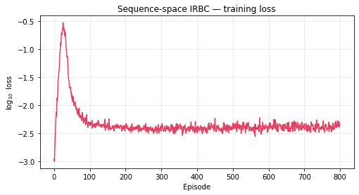

11.2 Ergodic distribution of $(k_1, k_2)$ ¶

Should concentrate near $(k_{ss}, k_{ss}) = (1, 1)$ with spread set by the AR(1) productivity dynamics. Compare visually to nb 01’s sim_periods scatter.

plt.figure(figsize=(7, 6))
xn = x_final.numpy() if isinstance(x_final, tf.Tensor) else x_final
plt.scatter(xn[:, 0], xn[:, 1], s=6, alpha=0.35, color='crimson')
plt.axvline(k_ss, color='k', linestyle=':', alpha=0.4)
plt.axhline(k_ss, color='k', linestyle=':', alpha=0.4)
plt.scatter([k_ss], [k_ss], color='black', marker='x', s=120, zorder=5, label='Steady state')
plt.xlabel('$k_1$'); plt.ylabel('$k_2$')
plt.title('Ergodic cloud after training (sequence-space IRBC)')
plt.legend(); plt.grid(True, alpha=0.3)
plt.show()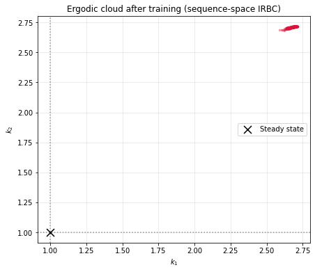

11.3 Per-equation residuals¶

Like nb 01’s Approach-C diagnostics. On this budget, residuals are comparable to the state-space DEQN — in fact often modestly better, because the SS-centred $\tanh$ parametrization acts as a strong prior near the stochastic steady state. FB residuals stay small since $\mu_j \approx 0$ on the ergodic set (irreversibility almost never binds at $\kappa = 0.5$ ).

loss_final, eul, arc, fbs = compute_residuals(x_final, h_final, nn)
print(f"Test loss on last cloud: {loss_final.numpy():.3e}\n")
print("Per-equation residuals (mean |.|, max |.|):")
for j in range(N_COUNTRIES):
    e = np.abs(eul[j].numpy())
    print(f"  Euler {j+1}:  mean = {e.mean():.2e},  max = {e.max():.2e}")
a = np.abs(arc.numpy())
print(f"  ARC    :  mean = {a.mean():.2e},  max = {a.max():.2e}")
for j in range(N_COUNTRIES):
    f = np.abs(fbs[j].numpy())
    print(f"  FB   {j+1}:  mean = {f.mean():.2e},  max = {f.max():.2e}")

Test loss on last cloud: 4.262e-03

Per-equation residuals (mean |.|, max |.|):
  Euler 1:  mean = 2.47e-02,  max = 9.26e-02
  Euler 2:  mean = 2.47e-02,  max = 9.29e-02
  ARC    :  mean = 3.66e-02,  max = 1.93e-01
  FB   1:  mean = 9.67e-03,  max = 2.24e-01
  FB   2:  mean = 5.90e-03,  max = 7.63e-02

11.4 Policy scatter¶

Comparable to nb 01’s “Capital Policy” panel — plot $k'_j$ vs $k_j$ on the ergodic cloud. The cloud here has narrower support in $k$ than the uniform-sampled cloud in nb 01, so we see a tighter scatter; but the 45-degree line is still the relevant reference.

raw_final = nn(h_final).numpy()
pol_final = policy_from_rates(x_final, nn(h_final)).numpy()
xn = x_final.numpy() if isinstance(x_final, tf.Tensor) else x_final

fig, axes = plt.subplots(1, 2, figsize=(12, 5))
for j, ax in enumerate(axes):
    ax.scatter(xn[:, j], pol_final[:, j], s=6, alpha=0.35,
               color=['crimson', 'steelblue'][j], label=f'$k\'_{j+1}$ (seq-space)')
    k_rng = np.linspace(xn[:, j].min(), xn[:, j].max(), 10)
    ax.plot(k_rng, k_rng, 'k--', alpha=0.5, label='45-deg')
    ax.set_xlabel(f'$k_{j+1}$'); ax.set_ylabel(f"$k'_{j+1}$")
    ax.set_title(f"Country {j+1}: $k'$ vs $k$")
    ax.legend(); ax.grid(True, alpha=0.3)
plt.tight_layout(); plt.show()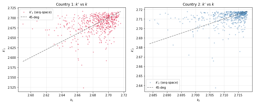

12. Take-away¶

The single conceptual change versus Day 3 nb 01’s state-space DEQN:

Day 3 nb 01 (state-space)	This notebook (sequence-space)
Network input: $(k_1, k_2, z_1, z_2)$ — 4 floats.	Network input: $\mathcal{E}_t^{(80)}$ — 240 floats.
Output head: `softplus` for all 5 policies (works because current $k$ is input).	Output head: SS-centred $\tanh$ for $k'_j, \lambda$ ; shifted softplus for $\mu_j$ .
Pre-training target: $(k_{ss}, k_{ss}, \lambda_{ss}, \varepsilon, \varepsilon)$ .	Pre-training target: raw output = 0 (parametrization does the rest).
Euler / ARC / FB residuals.	Unchanged.
Gauss–Hermite quadrature.	Unchanged.
Cloud-method sampling.	Unchanged, but the cloud carries a history alongside the state.

When does sequence space pay off?¶

BM (nb 05): 2-dim state, 1 shock → 25-dim history. Larger input. Pedagogical device only.
IRBC (this nb): 4-dim state, 3 shocks → 240-dim history. Much larger input. Still pedagogical — a bridge to KS.
Krusell–Smith (nb 06): infinite-dim state (wealth distribution), 1 shock → 100-dim history. First genuine win: exogenous input replaces the distribution summary statistics that state-space methods rely on.

The point of running IRBC in sequence space is not computational efficiency — it’s to show that the same training template works for a multi-equation system with multiple independent shock channels, before we hand the method over to Krusell–Smith where the real motivation kicks in.

What the residual comparison tells us¶

On this classroom budget the sequence-space network reaches residual levels comparable to (and in places better than) nb 01’s Approach C. Two forces partly offset each other:

Against sequence space: the network has to infer $(k_j, z_j)$ from a noisy 240-dim history rather than read them off as inputs. All else equal, residuals should be larger.
For sequence space: the SS-centred $\tanh$ parametrization injects a strong prior that the policy is near the steady state — nb 01’s softplus head has no such anchor. Combined with exponential LR decay this dominates the budget here.

Takeaway: sequence space is not automatically worse. At the scale where it matters (Krusell–Smith), the cost of inferring state from history is offset by the radically simpler input geometry.

Reference¶

Azinovic-Yang, M. & Žemlička, J. (2025). Deep Learning in the Sequence Space. arXiv:2509.13623. Companion JAX repository: azinoma/DeepLearningInTheSequenceSpace.