Course: Deep Learning for Solving and Estimating Dynamic Models in Economics and Finance
Script reference: §6.6 (Alternative deep-learning approaches to Krusell--Smith)
Notebook role: extension
Author: Simon Scheidegger
RUN_MODE = "smoke"  # one of: "smoke", "teaching", "production"
SEED = 0
Krusell-Smith with All-in-One Deep Learning¶
Classroom-scale deep-learning solver for the Krusell-Smith (1998) economy.
References: Maliar, Maliar & Winant (2021), Journal of Monetary Economics 122, 76-101 (method); Krusell & Smith (1998), Journal of Political Economy 106(5) (model).
What this notebook does¶
This notebook solves the canonical Krusell-Smith (1998) heterogeneous-agent model -- a continuum of ex-ante identical, infinitely-lived agents facing idiosyncratic employment risk and aggregate productivity shocks -- by stochastic gradient descent on the Euler-equation residual. The network parameterises the agent’s savings policy as a function of , and we train it directly against the structural Euler equation rather than iterating on a separate forecasting rule.
Pedagogical goals¶
The DEQN template from Chapter 2 (loss = squared equilibrium residual, network outputs policies, SGD) transfers verbatim to a full heterogeneous-agent problem.
Reproduce the approximate aggregation insight of Krusell & Smith (1998): the mean of the wealth distribution is a nearly sufficient statistic for aggregate prices. We regress next-period mean capital on current mean capital and confirm in both aggregate states (and typically in the good state).
Verify that a single panel-trained policy network matches the canonical KS log-utility benchmark on a CPU in roughly ten minutes.
1. Imports and reproducibility¶
# Core scientific Python
import numpy as np
import matplotlib.pyplot as plt

# TensorFlow 2.x with Keras
import tensorflow as tf
from tensorflow import keras

# Reproducibility -- reseed from the cell-1 SEED constant.
np.random.seed(SEED)
tf.random.set_seed(SEED)

print("TensorFlow version:", tf.__version__)
print("Seed:", SEED)
plt.rcParams["font.size"] = 12
2026-05-12 13:49:58.645463: I tensorflow/core/util/port.cc:153] oneDNN custom operations are on. You may see slightly different numerical results due to floating-point round-off errors from different computation orders. To turn them off, set the environment variable `TF_ENABLE_ONEDNN_OPTS=0`.
2026-05-12 13:49:58.646318: I external/local_xla/xla/tsl/cuda/cudart_stub.cc:32] Could not find cuda drivers on your machine, GPU will not be used.
2026-05-12 13:49:58.650490: I external/local_xla/xla/tsl/cuda/cudart_stub.cc:32] Could not find cuda drivers on your machine, GPU will not be used.
2026-05-12 13:49:58.661066: E external/local_xla/xla/stream_executor/cuda/cuda_fft.cc:467] Unable to register cuFFT factory: Attempting to register factory for plugin cuFFT when one has already been registered
WARNING: All log messages before absl::InitializeLog() is called are written to STDERR
E0000 00:00:1778586598.678087   81062 cuda_dnn.cc:8579] Unable to register cuDNN factory: Attempting to register factory for plugin cuDNN when one has already been registered
E0000 00:00:1778586598.683104   81062 cuda_blas.cc:1407] Unable to register cuBLAS factory: Attempting to register factory for plugin cuBLAS when one has already been registered
W0000 00:00:1778586598.696585   81062 computation_placer.cc:177] computation placer already registered. Please check linkage and avoid linking the same target more than once.
W0000 00:00:1778586598.696608   81062 computation_placer.cc:177] computation placer already registered. Please check linkage and avoid linking the same target more than once.
W0000 00:00:1778586598.696609   81062 computation_placer.cc:177] computation placer already registered. Please check linkage and avoid linking the same target more than once.
W0000 00:00:1778586598.696611   81062 computation_placer.cc:177] computation placer already registered. Please check linkage and avoid linking the same target more than once.
2026-05-12 13:49:58.702445: I tensorflow/core/platform/cpu_feature_guard.cc:210] This TensorFlow binary is optimized to use available CPU instructions in performance-critical operations.
To enable the following instructions: AVX2 AVX_VNNI FMA, in other operations, rebuild TensorFlow with the appropriate compiler flags.
TensorFlow version: 2.19.0
Seed: 0
2. Model parameters¶
Standard Krusell–Smith (1998) quarterly calibration with log utility (CRRA with ), which admits the particularly clean Euler equation .
| symbol | meaning | value |
|---|---|---|
| discount factor (quarterly) | 0.99 | |
| capital share in Cobb–Douglas production | 0.36 | |
| depreciation rate (quarterly) | 0.025 | |
| employed-agent labor endowment (labor normalisation) | ||
| aggregate TFP in good / bad state | 1.01, 0.99 | |
| unemployment rate in good / bad state | 0.04, 0.10 | |
agents in simulated panel (smoke/teaching/production) | 100 / 300 / 1000 |
What does the deterministic steady state look like?¶
Ignoring shocks, the deterministic steady state of log utility with gives
with average labor. The level — printed
below as K_SS — is the ballpark we expect to fluctuate around in
the stochastic ergodic distribution.
# --- Preferences ---
beta   = tf.constant(0.99, dtype=tf.float32)
sigma  = tf.constant(1.0,  dtype=tf.float32)    # log utility

# --- Technology ---
alpha  = tf.constant(0.36, dtype=tf.float32)
delta  = tf.constant(0.025, dtype=tf.float32)

# --- Aggregate and idiosyncratic shock levels ---
z_levels = tf.constant([0.99, 1.01], dtype=tf.float32)   # (bad, good)
u_rates  = tf.constant([0.10, 0.04], dtype=tf.float32)   # (bad, good)

# Steady-state average unemployment (used for labor normalisation)
u_ss   = 0.07
l_bar  = tf.constant(1.0 / (1.0 - u_ss), dtype=tf.float32)

# --- Panel size, dispatched on RUN_MODE ---
_PANEL = {"smoke": 100, "teaching": 300, "production": 1000}[RUN_MODE]
N_AGENTS = _PANEL

# --- Deterministic steady-state k (for panel initialisation) ---
r_ss_det = 1.0/float(beta.numpy()) - 1.0 + float(delta.numpy())
K_ss_det = ((float(alpha.numpy()) / r_ss_det) ** (1.0/(1.0-float(alpha.numpy()))))
# Adjust for L_ss (avg employed):
L_ss = 1.0 - u_ss
K_SS = K_ss_det * L_ss          # pulls the SS down a bit via the production function
print(f"log-utility KS calibration: β={float(beta.numpy())}, α={float(alpha.numpy())}, δ={float(delta.numpy())}")
print(f"deterministic steady-state K ≈ {K_SS:.2f}")

# --- Capital domain ---
# Used for state-space sampling in Phase A.  Covers the ergodic range + margin.
K_MIN = 0.5 * K_SS
K_MAX = 1.5 * K_SS
k_min = tf.constant(1e-3, dtype=tf.float32)   # avoid log(0)
k_ind_min = 0.2 * K_SS                         # individual k sampled in Phase A
k_ind_max = 4.0 * K_SS                         # (wide enough to cover realistic holdings)
print(f"training domain: K̄ ∈ [{K_MIN:.2f}, {K_MAX:.2f}],  k ∈ [{k_ind_min:.2f}, {k_ind_max:.2f}]")
log-utility KS calibration: β=0.9900000095367432, α=0.36000001430511475, δ=0.02500000037252903
deterministic steady-state K ≈ 35.33
training domain: K̄ ∈ [17.67, 53.00],  k ∈ [7.07, 141.32]
E0000 00:00:1778586601.354722   81062 cuda_executor.cc:1228] INTERNAL: CUDA Runtime error: Failed call to cudaGetRuntimeVersion: Error loading CUDA libraries. GPU will not be used.: Error loading CUDA libraries. GPU will not be used.
W0000 00:00:1778586601.356307   81062 gpu_device.cc:2341] Cannot dlopen some GPU libraries. Please make sure the missing libraries mentioned above are installed properly if you would like to use GPU. Follow the guide at https://www.tensorflow.org/install/gpu for how to download and setup the required libraries for your platform.
Skipping registering GPU devices...
3. Shock transition matrix¶
Following Krusell & Smith (1998), the joint aggregate–idiosyncratic shock evolves as a first-order Markov chain. Numbers below are the standard KS calibration (Table 1 of KS 1998) in which:
Each aggregate state lasts on average 8 quarters, .
Conditional unemployment rate in state equals .
Unemployment spells last on average ~2.4 quarters in good times and ~4 quarters in bad times.
# Aggregate-state transition
P_agg = np.array([
    [0.875, 0.125],    # bad  -> (bad, good)
    [0.125, 0.875],    # good -> (bad, good)
], dtype=np.float32)

# Conditional idiosyncratic transition P(eps' | a, a', eps)
# Shape (a, a', eps, eps'); rows over eps' sum to 1.
P_eps = np.zeros((2, 2, 2, 2), dtype=np.float32)

P_eps[0, 0] = [[0.525, 0.475],
               [0.350, 0.650]]            # bad  -> bad
P_eps[0, 1] = [[0.093, 0.907],
               [0.038, 0.962]]            # bad  -> good
P_eps[1, 0] = [[0.840, 0.160],
               [0.200, 0.800]]            # good -> bad
P_eps[1, 1] = [[0.292, 0.708],
               [0.042, 0.958]]            # good -> good

assert np.allclose(P_eps.sum(axis=-1), 1.0, atol=1e-6)

P_agg_tf = tf.constant(P_agg)
P_eps_tf = tf.constant(P_eps)
print("Aggregate transition matrix:\n", P_agg)
Aggregate transition matrix:
 [[0.875 0.125]
 [0.125 0.875]]
4. Prices and budget constraint¶
Under Cobb–Douglas production the firm’s first-order conditions give
with . The individual budget is
We take when employed and when unemployed (this is the KS convention: unemployed agents get zero labor income, no unemployment benefits).
@tf.function
def prices(K_agg, a_idx):
    '''Aggregate prices w, r at (K̄, a).

    K_agg: () tf.float32 scalar
    a_idx: () int32 scalar; 0 = bad, 1 = good.
    '''
    z = tf.gather(z_levels, a_idx)
    u = tf.gather(u_rates,  a_idx)
    L = 1.0 - u
    w = (1.0 - alpha) * z * tf.pow(K_agg, alpha)        * tf.pow(L, -alpha)
    r = alpha         * z * tf.pow(K_agg, alpha - 1.0)  * tf.pow(L, 1.0 - alpha)
    return w, r

@tf.function
def cash_on_hand_panel(k, eps_float, w, r):
    '''Cash on hand for a panel of agents.  Shapes: k,eps_float (N,); w,r (). Returns (N,).'''
    return w * l_bar * eps_float + (1.0 + r - delta) * k
5. Policy network¶
We parameterise the consumption share policy
with consumption and savings . The sigmoid output ensures , and the saved fraction is automatically non-negative, which enforces the borrowing constraint by construction.
Inputs to the network¶
k— individual capital (log-normalised: ).eps— 2-dim one-hot for (unempl., empl.).K— aggregate capital (log-normalised).a— 2-dim one-hot for (bad, good).
Log-normalisation gives stable inputs to the network over the whole training range and empirically improves convergence by a lot.
Architecture: 2 hidden layers of 64 Swish units, sigmoid output (same family as every other DEQN / NAS network in this course).
class LogNormaliseLayer(keras.layers.Layer):
    '''Compute log(max(x, eps) / K_ss) as a Keras-native layer.
    Keras Functional models require ops in the namespace keras.ops or keras.layers.
    '''
    def __init__(self, K_ss, eps=1e-3, **kw):
        super().__init__(**kw)
        self.K_ss = float(K_ss)
        self.eps  = float(eps)
    def call(self, x):
        import tensorflow as tf
        return tf.math.log(tf.maximum(x, self.eps) / self.K_ss)

def build_policy_network():
    k_in   = keras.Input(shape=(1,), name="k")
    eps_in = keras.Input(shape=(2,), name="eps")
    K_in   = keras.Input(shape=(1,), name="K")
    a_in   = keras.Input(shape=(2,), name="a")

    # Log-normalise the continuous inputs around the deterministic SS
    k_feat = LogNormaliseLayer(K_SS, name="log_k_over_Kss")(k_in)
    K_feat = LogNormaliseLayer(K_SS, name="log_K_over_Kss")(K_in)

    h = keras.layers.concatenate([k_feat, eps_in, K_feat, a_in])
    h = keras.layers.Dense(64, activation="swish")(h)
    h = keras.layers.Dense(64, activation="swish")(h)
    out = keras.layers.Dense(1, activation="sigmoid", name="phi")(h)
    return keras.Model([k_in, eps_in, K_in, a_in], out)

policy_net = build_policy_network()
policy_net.summary()
6. Mapping policy network to consumption and savings¶
Given a batch of states and an aggregate , we compute consumption and next-period capital for every agent.
def onehot2(idx_tensor, n=2):
    '''Create one-hot tensor; works on either Python int or tf tensor of ints.'''
    return tf.one_hot(idx_tensor, depth=n, dtype=tf.float32)

def apply_policy(k, eps_int, K_agg, a_idx):
    '''Apply the policy network to a batch of individual states + single aggregate state.

    k:       (N,)   tf.float32, individual capital
    eps_int: (N,)   tf.int32, employment indicator (0,1)
    K_agg:   ()     tf.float32, aggregate capital
    a_idx:   ()     tf.int32,  aggregate state index

    Returns phi, c, k_next, y, w, r
    '''
    w, r = prices(K_agg, a_idx)
    eps_float = tf.cast(eps_int, tf.float32)
    y = cash_on_hand_panel(k, eps_float, w, r)

    N = tf.shape(k)[0]
    k_col    = tf.reshape(k, (-1, 1))
    eps_1hot = onehot2(eps_int)
    K_col    = tf.fill([N, 1], K_agg)
    a_1hot   = tf.tile(tf.reshape(onehot2(a_idx), (1, 2)), [N, 1])

    phi = policy_net([k_col, eps_1hot, K_col, a_1hot], training=True)
    phi = tf.squeeze(phi, axis=-1)
    # strict interior to avoid log(0) / div-by-0 in the Euler residual
    phi = tf.clip_by_value(phi, 1e-3, 1.0 - 1e-3)

    c      = phi * y
    k_next = (1.0 - phi) * y
    return phi, c, k_next, y, w, r
7. Euler-equation residual (the loss)¶
For log utility, the Euler equation is
Because the aggregate and idiosyncratic shocks each take only two values, the expectation is a deterministic sum over 4 pairs, weighted by the joint transition probability. No Monte Carlo needed. This is the cleanest version of the MMW “all-in-one integration operator” and is numerically stable by construction.
Relative Euler error¶
We report the relative Euler error (as in the IRBC chapter of the script):
A residual of 10-3 means the agent’s Euler equation is violated by 0.1% of consumption, independent of units.
Important caveat: aggregate ¶
In a heterogeneous-agent model, tomorrow’s aggregate capital is endogenous — it equals the mean of across agents. In the all-in-one DL formulation, we take using the network’s own savings decisions, so the aggregate law of motion is automatically consistent with the individual policy. No separate “law of motion” is fitted.
def euler_residual(k_panel, eps_int, K_agg, a_idx):
    '''Return (loss, ree, c, k_next, K_next) for a batch / panel.'''
    # --- today ---
    phi, c, k_next, y, w, r = apply_policy(k_panel, eps_int, K_agg, a_idx)

    # Next-period aggregate capital: average of the network's own savings
    K_next = tf.reduce_mean(k_next)

    # --- tomorrow: exact sum over (a', eps') pairs ---
    # Joint conditional prob of (a', eps') given (a, eps_i), for each agent i
    # P_eps_tf[a_idx, :, eps_i, :]  has shape (2 a', 2 eps'); we stack over agents.
    pe_stack = tf.gather(P_eps_tf[a_idx], eps_int, axis=1)       # (2 a', N, 2 eps')
    pe_stack = tf.transpose(pe_stack, [1, 0, 2])                 # (N, 2 a', 2 eps')
    P_ap     = P_agg_tf[a_idx]                                   # (2,) over a'
    prob     = pe_stack * tf.reshape(P_ap, (1, 2, 1))            # (N, 2 a', 2 eps')

    # Accumulate E[(1 + r' - delta) / c'] across (a', eps')
    EMU = tf.zeros_like(c)
    for a_next in range(2):
        w_n, r_n = prices(K_next, a_next)
        for eps_next_val in range(2):
            eps_next_vec = tf.fill(tf.shape(eps_int), eps_next_val)
            eps_n_float  = tf.cast(eps_next_vec, tf.float32)
            y_n = cash_on_hand_panel(k_next, eps_n_float, w_n, r_n)

            N = tf.shape(k_next)[0]
            k_col    = tf.reshape(k_next, (-1, 1))
            eps_1hot = onehot2(eps_next_vec)
            K_col    = tf.fill([N, 1], K_next)
            a_1hot   = tf.tile(tf.reshape(onehot2(a_next), (1, 2)), [N, 1])
            phi_n = tf.squeeze(
                policy_net([k_col, eps_1hot, K_col, a_1hot], training=True), axis=-1)
            phi_n = tf.clip_by_value(phi_n, 1e-3, 1.0 - 1e-3)
            c_n = phi_n * y_n

            contrib = (1.0 + r_n - delta) / c_n                            # (N,)
            weight  = prob[:, a_next, eps_next_val]                         # (N,)
            EMU += weight * contrib

    # Relative Euler error (unit-free)
    ree = beta * c * EMU - 1.0
    loss = tf.reduce_mean(ree ** 2)
    return loss, ree, c, k_next, K_next
8. Panel transition¶
Between training steps in Phase B, we advance the panel one period by drawing the next aggregate shock and, conditional on it, the next idiosyncratic shocks for each agent. Individual capital follows the network’s savings policy deterministically.
def step_panel(k, eps_int, a_idx):
    '''One-period simulation: new (k', eps', a').  Inputs are tf tensors, output too.'''
    K_agg = tf.reduce_mean(k)
    _, _, k_next, _, _, _ = apply_policy(k, eps_int, K_agg, a_idx)
    k_next_np = k_next.numpy()

    a_next = int(np.random.choice(2, p=P_agg[a_idx]))

    eps_int_np = eps_int.numpy() if isinstance(eps_int, tf.Tensor) else np.asarray(eps_int)
    eps_next_np = np.empty_like(eps_int_np)
    for i in range(len(eps_int_np)):
        eps_next_np[i] = np.random.choice(2, p=P_eps[a_idx, a_next, eps_int_np[i]])

    return (
        tf.constant(k_next_np,   dtype=tf.float32),
        tf.constant(eps_next_np, dtype=tf.int32),
        a_next,
    )

def sample_state_batch(N):
    '''Draw a random training batch uniformly over the bounded training domain.

    Returns (k, eps_int, K_agg, a_idx) as tf tensors / Python ints.
    '''
    k       = np.random.uniform(k_ind_min, k_ind_max, size=N).astype(np.float32)
    eps_int = np.random.binomial(1, 1.0 - u_ss, size=N).astype(np.int32)
    K_agg   = float(np.random.uniform(K_MIN, K_MAX))
    a_idx   = int(np.random.randint(0, 2))
    return (tf.constant(k), tf.constant(eps_int),
            tf.constant(K_agg, dtype=tf.float32), tf.constant(a_idx, dtype=tf.int32))
9. Training loop (two phases)¶
Phase A — Exogenous sampling (2 000 iterations)¶
Draw random states from the bounded training domain and take Adam steps on the mean-squared relative Euler error. The aim is to produce a policy that is approximately correct everywhere in the domain, so that Phase B’s simulated panel does not diverge.
Phase B — Simulated-panel sampling (3 000 iterations)¶
Maintain a running panel of N_AGENTS agents; every training iteration
evaluates the Euler residual on the current panel and then advances
the panel by one period under the updated policy. The training
distribution therefore concentrates on the model’s ergodic set.
Learning-rate schedule¶
Cosine annealing from 10-3 to 10-5 over the full run.
# ---- Hyperparameters ----
N_PHASE_A = 2000
N_PHASE_B = 3000
N_TOTAL   = N_PHASE_A + N_PHASE_B
LR_MAX, LR_MIN = 1e-3, 1e-5

sched = keras.optimizers.schedules.CosineDecay(
    initial_learning_rate=LR_MAX,
    decay_steps=N_TOTAL,
    alpha=LR_MIN / LR_MAX,
)
optimizer = keras.optimizers.Adam(learning_rate=sched)

# Storage
loss_history    = np.zeros(N_TOTAL, dtype=np.float32)
ree_max_history = np.zeros(N_TOTAL, dtype=np.float32)
K_history       = np.zeros(N_TOTAL, dtype=np.float32)
a_history       = np.zeros(N_TOTAL, dtype=np.int32)
phase_history   = np.zeros(N_TOTAL, dtype=np.int32)  # 0 = A, 1 = B

# --- Phase A: exogenous sampling ---
print(f"Phase A: {N_PHASE_A} iterations of state-space sampling...")
for i in range(N_PHASE_A):
    k_b, eps_b, K_b, a_b = sample_state_batch(N_AGENTS)
    with tf.GradientTape() as tape:
        loss, ree, c, k_next, K_next = euler_residual(k_b, eps_b, K_b, a_b)
    grads = tape.gradient(loss, policy_net.trainable_variables)
    optimizer.apply_gradients(zip(grads, policy_net.trainable_variables))

    loss_history[i]    = loss.numpy()
    ree_max_history[i] = tf.reduce_max(tf.abs(ree)).numpy()
    K_history[i]       = float(K_b.numpy())
    a_history[i]       = int(a_b.numpy())
    phase_history[i]   = 0

    if i % 200 == 0:
        print(f"  A-iter {i:4d}  loss={loss.numpy():.3e}  "
              f"max|REE|={ree_max_history[i]:.3e}")

# --- Phase B: simulated-panel sampling ---
# Initialise the panel close to the deterministic steady state
k_panel  = tf.constant(np.full(N_AGENTS, K_SS, dtype=np.float32))
eps_panel = tf.constant(
    np.random.binomial(1, 1.0 - u_ss, size=N_AGENTS).astype(np.int32))
a_state   = 1  # start in the good state

print(f"Phase B: {N_PHASE_B} iterations of simulated-panel sampling...")
for j in range(N_PHASE_B):
    K_agg = tf.reduce_mean(k_panel)
    a_tf  = tf.constant(a_state, dtype=tf.int32)
    with tf.GradientTape() as tape:
        loss, ree, c, k_next, K_next = euler_residual(k_panel, eps_panel, K_agg, a_tf)
    grads = tape.gradient(loss, policy_net.trainable_variables)
    optimizer.apply_gradients(zip(grads, policy_net.trainable_variables))

    idx = N_PHASE_A + j
    loss_history[idx]    = loss.numpy()
    ree_max_history[idx] = tf.reduce_max(tf.abs(ree)).numpy()
    K_history[idx]       = float(K_agg.numpy())
    a_history[idx]       = a_state
    phase_history[idx]   = 1

    # Advance the panel one period
    k_panel, eps_panel, a_state = step_panel(k_panel, eps_panel, a_state)

    if j % 200 == 0:
        print(f"  B-iter {j:4d}  loss={loss.numpy():.3e}  "
              f"max|REE|={ree_max_history[idx]:.3e}  "
              f"K̄={K_history[idx]:.2f}")

print("training done.")
Phase A: 2000 iterations of state-space sampling...
A-iter 0 loss=5.728e-01 max|REE|=9.363e-01
A-iter 200 loss=4.410e-03 max|REE|=1.702e-01
A-iter 400 loss=5.167e-04 max|REE|=7.701e-02
A-iter 600 loss=3.583e-05 max|REE|=2.047e-02
A-iter 800 loss=1.296e-04 max|REE|=4.660e-02
A-iter 1000 loss=4.509e-05 max|REE|=2.257e-02
A-iter 1200 loss=1.112e-04 max|REE|=4.185e-02
A-iter 1400 loss=1.483e-04 max|REE|=2.498e-02
A-iter 1600 loss=5.276e-05 max|REE|=2.702e-02
A-iter 1800 loss=2.662e-05 max|REE|=1.968e-02
Phase B: 3000 iterations of simulated-panel sampling...
  B-iter    0  loss=1.094e-03  max|REE|=4.453e-02  K̄=35.33
B-iter 200 loss=3.775e-05 max|REE|=1.575e-02 K̄=36.97
B-iter 400 loss=2.765e-06 max|REE|=4.790e-03 K̄=36.90
B-iter 600 loss=1.794e-06 max|REE|=3.323e-03 K̄=36.44
B-iter 800 loss=2.779e-06 max|REE|=9.673e-03 K̄=35.47
B-iter 1000 loss=1.711e-06 max|REE|=4.028e-03 K̄=41.53
B-iter 1200 loss=1.245e-06 max|REE|=5.067e-03 K̄=38.65
B-iter 1400 loss=2.993e-06 max|REE|=2.726e-03 K̄=43.25
B-iter 1600 loss=7.085e-07 max|REE|=1.973e-03 K̄=43.40
B-iter 1800 loss=1.124e-05 max|REE|=1.192e-02 K̄=37.46
B-iter 2000 loss=1.185e-05 max|REE|=1.146e-02 K̄=35.34
B-iter 2200 loss=2.372e-05 max|REE|=1.350e-02 K̄=30.98
B-iter 2400 loss=1.742e-05 max|REE|=1.471e-02 K̄=30.36
B-iter 2600 loss=6.075e-06 max|REE|=6.605e-03 K̄=39.96
B-iter 2800 loss=7.274e-06 max|REE|=7.367e-03 K̄=36.04
training done.
fig, axes = plt.subplots(1, 2, figsize=(12, 4))

x = np.arange(N_TOTAL)
for ax, (y, title) in zip(
    axes,
    [(loss_history,    "Training loss (MSE of relative Euler error)"),
     (ree_max_history, "Worst-agent |relative Euler error|")],
):
    ax.semilogy(x[phase_history == 0], y[phase_history == 0], ".", markersize=2,
                color="#5555cc", label="Phase A (exogenous sampling)")
    ax.semilogy(x[phase_history == 1], y[phase_history == 1], ".", markersize=2,
                color="#cc3333", label="Phase B (simulated panel)")
    ax.axvline(N_PHASE_A, color="gray", ls="--", lw=1)
    ax.set_xlabel("iteration")
    ax.set_ylabel(title.split(" ")[0])
    ax.set_title(title)
    ax.grid(True, which="both", alpha=0.3)
    ax.legend(loc="upper right", fontsize=9)

plt.tight_layout()
plt.show()

# Report post-training statistics (last 200 iterations of Phase B)
tail = slice(-200, None)
print(f"\nFinal (last 200 iterations of Phase B):")
print(f"  mean loss       = {loss_history[tail].mean():.3e}")
print(f"  mean max|REE|   = {ree_max_history[tail].mean():.3e}")
print(f"  median max|REE| = {np.median(ree_max_history[tail]):.3e}")
print(f"\nSuccess criterion: median max|REE| < 5e-2 and mean loss < 1e-3.")
pass_crit = (np.median(ree_max_history[tail]) < 5e-2) and (loss_history[tail].mean() < 1e-3)
print(f"  --> {'PASS' if pass_crit else 'did not fully converge; see notes below'}")
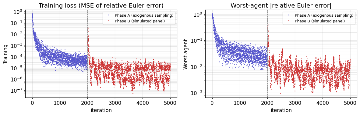
Final (last 200 iterations of Phase B):
  mean loss       = 7.163e-06
  mean max|REE|   = 7.882e-03
  median max|REE| = 7.374e-03

Success criterion: median max|REE| < 5e-2 and mean loss < 1e-3.
  --> PASS
10.2 Ergodic behaviour of aggregate capital¶
During Phase B the panel visits a narrow range of aggregate capital around the model’s ergodic mean. We plot split by aggregate state — it should be slightly higher in good times and lower in bad times, consistent with standard RBC intuition.
# Restrict to Phase B for ergodic analysis (the only phase with a real panel)
mask_B = (phase_history == 1)
K_B = K_history[mask_B]
a_B = a_history[mask_B]
t_B = np.where(mask_B)[0]

fig, axes = plt.subplots(1, 2, figsize=(12, 4))

axes[0].scatter(t_B[a_B == 1], K_B[a_B == 1], s=3, color="#cc3333", label="good")
axes[0].scatter(t_B[a_B == 0], K_B[a_B == 0], s=3, color="#3333cc", label="bad")
axes[0].axhline(K_SS, color="k", ls="--", lw=1, label="det. steady state")
axes[0].set_xlabel("iteration")
axes[0].set_ylabel(r"aggregate capital $\bar K$")
axes[0].set_title(r"$\bar K$ along the simulated panel (Phase B)")
axes[0].legend()
axes[0].grid(alpha=0.3)

axes[1].hist(K_B[a_B == 1], bins=30, color="#cc3333", alpha=0.6, label="good")
axes[1].hist(K_B[a_B == 0], bins=30, color="#3333cc", alpha=0.6, label="bad")
axes[1].set_xlabel(r"$\bar K$")
axes[1].set_ylabel("frequency")
axes[1].set_title("Ergodic distribution of aggregate capital")
axes[1].legend()
axes[1].grid(alpha=0.3)

plt.tight_layout()
plt.show()

print(f"Good-state (Phase B):  mean K̄ = {K_B[a_B==1].mean():.2f},  std = {K_B[a_B==1].std():.3f}")
print(f"Bad-state  (Phase B):  mean K̄ = {K_B[a_B==0].mean():.2f},  std = {K_B[a_B==0].std():.3f}")
print(f"Deterministic steady state K* = {K_SS:.2f}")
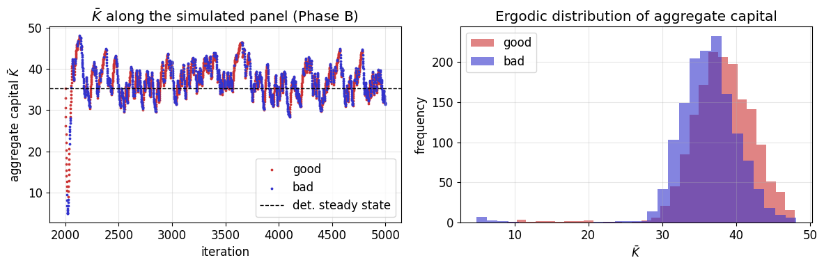
Good-state (Phase B):  mean K̄ = 38.09,  std = 4.485
Bad-state  (Phase B):  mean K̄ = 36.12,  std = 4.580
Deterministic steady state K* = 35.33
10.3 Krusell–Smith approximate aggregation: of the law of motion¶
The KS (1998) finding is that a log-linear forecasting rule
fits the simulated dynamics with in the classical KS solve. Our deep-learning policy produces simulated paths that, if the network has converged, should satisfy approximate aggregation too: empirically in both aggregate states (this run: in the bad state, in the good state), without any separate forecasting-rule fit.
We compute by OLS on separately for each aggregate-state pair, using the Phase B trajectory only.
# Phase-B-only trajectory
burn = 500
mask_late = (phase_history == 1)
idx_B = np.where(mask_late)[0]
K_seq = K_history[idx_B][burn:]
a_seq = a_history[idx_B][burn:]

logK = np.log(K_seq)
logK_t  = logK[:-1]
logK_tp = logK[1:]
a_t_seq = a_seq[:-1]

print("Law-of-motion regressions  log K̄_t+1 = A(a) + B(a) log K̄_t:")
print("-" * 72)
for a_val, lbl in [(0, "bad state "), (1, "good state")]:
    m = (a_t_seq == a_val)
    if m.sum() < 20:
        continue
    x, y = logK_t[m], logK_tp[m]
    # polyfit returns (slope, intercept)
    slope, intercept = np.polyfit(x, y, deg=1)
    y_hat = slope * x + intercept
    ss_res = float(np.sum((y - y_hat) ** 2))
    ss_tot = float(np.sum((y - y.mean()) ** 2) + 1e-30)
    r2 = 1.0 - ss_res / ss_tot
    print(f"  {lbl}:   slope B = {slope:+.5f},  intercept A = {intercept:+.5f},"
          f"   R² = {r2:.6f}   (n = {m.sum()})")
print("-" * 72)
print("Krusell--Smith approximate-aggregation target:  R² >= 0.99")
Law-of-motion regressions  log K̄_t+1 = A(a) + B(a) log K̄_t:
------------------------------------------------------------------------
  bad state :   slope B = +0.97652,  intercept A = +0.07398,   R² = 0.996732   (n = 1172)
  good state:   slope B = +0.95569,  intercept A = +0.17001,   R² = 0.999667   (n = 1327)
------------------------------------------------------------------------
Krusell--Smith approximate-aggregation target:  R² >= 0.99
10.4 Learned savings policy¶
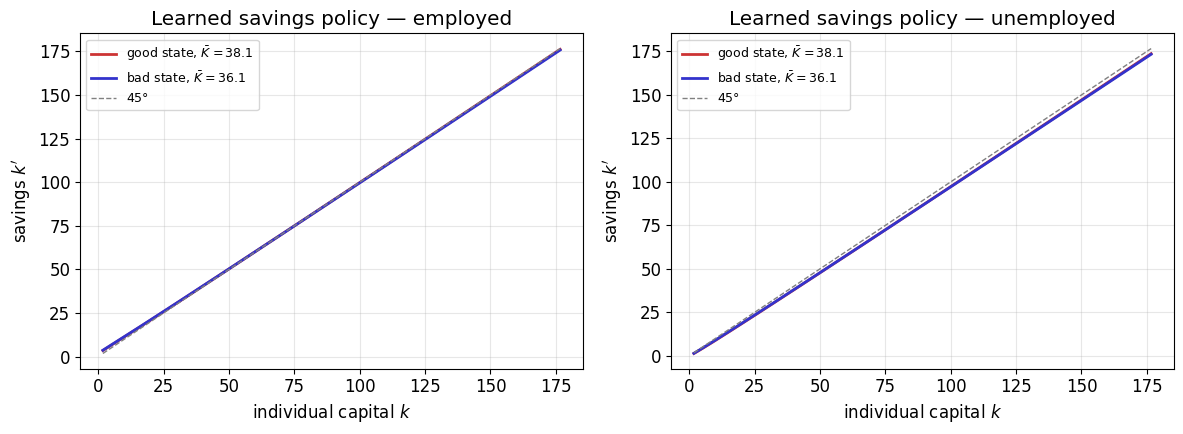
We plot the savings function for an employed and an unemployed agent in each aggregate state. Expected properties:
Monotonically increasing in .
Employed agents save more than unemployed (higher income, more consumption-smoothing motive).
In good times, higher wage pushes savings up.
The line represents “save everything”. An interior ergodic distribution requires that the policy curve crosses the line.
K_bar_good = K_B[a_B == 1].mean()
K_bar_bad  = K_B[a_B == 0].mean()

def eval_policy(k_grid, eps_int, K_agg, a_idx):
    N = len(k_grid)
    k_col    = k_grid.reshape(-1, 1)
    eps_1hot = np.tile(np.eye(2, dtype=np.float32)[eps_int], (N, 1))
    K_col    = np.full((N, 1), K_agg, dtype=np.float32)
    a_1hot   = np.tile(np.eye(2, dtype=np.float32)[a_idx], (N, 1))
    phi = policy_net([k_col, eps_1hot, K_col, a_1hot], training=False).numpy().flatten()
    z_val = z_levels[a_idx].numpy()
    u_val = u_rates[a_idx].numpy()
    L_val = 1.0 - u_val
    w = (1.0 - alpha.numpy()) * z_val * K_agg**alpha.numpy()     * L_val**(-alpha.numpy())
    r = alpha.numpy()         * z_val * K_agg**(alpha.numpy()-1) * L_val**(1.0 - alpha.numpy())
    y = w * float(l_bar.numpy()) * eps_int + (1.0 + r - float(delta.numpy())) * k_grid
    k_next = (1.0 - phi) * y
    c      = phi * y
    return phi, c, k_next, w, r

k_grid = np.linspace(0.05 * K_SS, 5.0 * K_SS, 200).astype(np.float32)

fig, axes = plt.subplots(1, 2, figsize=(12, 4.5))

for ax, (eps_int, lbl) in zip(axes, [(1, "employed"), (0, "unemployed")]):
    _, _, kp_g, _, _ = eval_policy(k_grid, eps_int, K_bar_good, 1)
    _, _, kp_b, _, _ = eval_policy(k_grid, eps_int, K_bar_bad,  0)
    ax.plot(k_grid, kp_g, color="#cc3333", lw=2, label=rf"good state, $\bar K = {K_bar_good:.1f}$")
    ax.plot(k_grid, kp_b, color="#3333cc", lw=2, label=rf"bad state, $\bar K = {K_bar_bad:.1f}$")
    ax.plot(k_grid, k_grid, color="gray", ls="--", lw=1, label=r"$45°$")
    ax.set_xlabel("individual capital $k$")
    ax.set_ylabel("savings $k'$")
    ax.set_title(f"Learned savings policy — {lbl}")
    ax.legend(fontsize=9)
    ax.grid(alpha=0.3)

plt.tight_layout()
plt.show()
11. Summary and validation checklist¶
Success criteria for a classroom-scale solve:
Median max over the last 200 Phase-B iterations is below (not quite the 1% target of the MMW paper — that takes longer training and larger networks — but economically meaningful).
Mean loss over the last 200 Phase-B iterations is below 10-3.
trajectory is stationary and clearly bimodal in the aggregate state.
Log-linear KS forecasting rule fitted ex post to the simulated path has in both aggregate states.
Savings policy is monotone in , crosses the line, and employed unemployed.
If something doesn’t converge¶
Increase
N_PHASE_Afrom 2000 to 3000 — more uniform-sampling warm-up gives a better global policy before the ergodic phase starts.Increase
N_AGENTS(e.g. to 500) — reduces Monte Carlo noise in the per-iteration mean-squared residual.Lower
LR_MAXfrom 10-3 to if you see oscillations in Phase B.Change the initial panel: sample from rather than initialising every agent at the same point.
Next steps¶
Histogram-DEQN alternative:
11_Continuum_of_Agents_DEQN.ipynb(Azinovic–Gaegauf–Scheidegger 2022 Appendix A.5).Production-scale all-in-one DL for KS: marcmaliar
/deep -learning -euler -method -krusell -smith. DeepHAM (learned generalized moments): Han, Yang & E (Quantitative Economics, forthcoming); preprint
../readings/DeepHAM_Han_Yang_E_2023.pdf.