Lecture 05, Notebook 02: Random Search NAS on a 10-D Regression - Deep Learning for Solving and Estimating Dynamic Models in Economics and Finance

Course: Deep Learning for Solving and Estimating Dynamic Models in Economics and Finance
Script reference: §4.1 (the hyperparameter space), §4.3 (random search; Bergstra & Bengio projection argument)
Notebook role: core
Author: Simon Scheidegger

RUN_MODE = "smoke"  # one of: "smoke", "teaching", "production"
SEED = 0

Accompanies Lecture 05 — Neural Architecture Search (slides: 04_Neural_Architecture_Search.pdf).

This is the first of two hands-on NAS examples for Lecture 05:

Notebook	Method	Testbed
`02_NAS_Random_Search_10D.ipynb` (this notebook)	Random Search, no external library	10-D analytical regression
`03_NAS_RandomSearch_Hyperband.ipynb`	Random Search + Successive Halving, from scratch	Genz Gaussian on $[0,1]^2$

This notebook demonstrates an easy, transparent form of Neural Architecture Search (NAS) without extra libraries — just TensorFlow/Keras and a bit of Python. We:

Define a 10-dimensional analytical regression task (synthetic data with noise).
Specify a large search space (depth, width, activations, optimizers, learning rates, batch sizes, normalization, dropout, etc.).
Use Random Search to sample candidate architectures and hyperparameters.
Train each candidate briefly and evaluate on a validation set.
Select the top 5 architectures by validation performance.
Retrain the top models longer on train+val and evaluate on the held-out test set.

The notebook is heavily commented for a ~45-minute walkthrough.

Why Random Search?¶

Random Search is a surprisingly strong baseline for hyperparameter/architecture tuning:

Scales trivially with search space size.
Parallelizable and easy to reason about.
Often outperforms naive grid search given the same budget (because many hyperparameters are low-sensitivity).

Other simple NAS strategies to mention (not implemented here):

Successive Halving / Hyperband: Early-stop poor performers aggressively.
Bayesian Optimization: Model the response surface to guide sampling.
Evolutionary Strategies: Mutate and select architectures over generations.

Here we focus on Random Search for clarity and reproducibility.

0. Setup¶

Imports, versions, and a few utility helpers.

import os, sys, math, random, json, time
from dataclasses import dataclass
from typing import Dict, Any

import numpy as np
import tensorflow as tf
from tensorflow import keras
from tensorflow.keras import layers

print("Python:", sys.version.split()[0])
print("TensorFlow:", tf.__version__)

# Reproducibility (best-effort; SEED is set in the run-mode-switch cell above).
# Note: TF GPU ops are not fully deterministic without TF_DETERMINISTIC_OPS=1
# and additional kernel-level configuration; CPU runs are deterministic.
random.seed(SEED)
np.random.seed(SEED)
tf.random.set_seed(SEED)

# Reduce TF verbosity
os.environ['TF_CPP_MIN_LOG_LEVEL'] = '2'
tf.get_logger().setLevel('ERROR')

1. Define a 10D analytical function and generate data¶

We create a nonlinear function on $x\in\mathbb{R}^{10}$ with interactions and noise:

y = \sin(x_1) + 0.5\,x_2^2 - 0.3\,x_3 x_4 + 0.1\,\exp(x_5) + 0.25\,\sin(2\pi x_6) + 0.2\,\tanh(x_7+x_8) - 0.15\,|x_9| + 0.1\,x_{10} + \varepsilon

(1)

where $x_i\sim \mathcal{N}(0,1)$ and noise $\varepsilon\sim \mathcal{N}(0,\sigma^2)$ with a modest $\sigma$ .

def analytical_function(X: np.ndarray, noise_std: float = 0.1) -> np.ndarray:
    """Compute target y for a 10D input X with shape (n, 10)."""
    x1,x2,x3,x4,x5,x6,x7,x8,x9,x10 = [X[:,i] for i in range(10)]
    y = (
        np.sin(x1)
        + 0.5 * (x2**2)
        - 0.3 * (x3 * x4)
        + 0.1 * np.exp(0.5 * x5)
        + 0.25 * np.sin(2 * np.pi * x6)
        + 0.2 * np.tanh(x7 + x8)
        - 0.15 * np.abs(x9)
        + 0.1 * x10
    )
    y += np.random.normal(0.0, noise_std, size=y.shape)
    return y.astype(np.float32)

def make_dataset(n_train=8000, n_val=1000, n_test=1000, noise_std=0.1):
    X_train = np.random.randn(n_train, 10).astype(np.float32)
    X_val   = np.random.randn(n_val, 10).astype(np.float32)
    X_test  = np.random.randn(n_test, 10).astype(np.float32)
    y_train = analytical_function(X_train, noise_std)
    y_val   = analytical_function(X_val, noise_std)
    y_test  = analytical_function(X_test, noise_std)
    return (X_train, y_train), (X_val, y_val), (X_test, y_test)

(X_train, y_train), (X_val, y_val), (X_test, y_test) = make_dataset()
X_train.shape, y_train.shape

((8000, 10), (8000,))

Standardization¶

We standardize inputs and targets (fit on train, apply to val/test).

from sklearn.preprocessing import StandardScaler

x_scaler = StandardScaler().fit(X_train)
y_scaler = StandardScaler().fit(y_train.reshape(-1,1))

X_train_s = x_scaler.transform(X_train).astype(np.float32)
X_val_s   = x_scaler.transform(X_val).astype(np.float32)
X_test_s  = x_scaler.transform(X_test).astype(np.float32)

y_train_s = y_scaler.transform(y_train.reshape(-1,1)).astype(np.float32).reshape(-1)
y_val_s   = y_scaler.transform(y_val.reshape(-1,1)).astype(np.float32).reshape(-1)
y_test_s  = y_scaler.transform(y_test.reshape(-1,1)).astype(np.float32).reshape(-1)

X_train_s.shape, y_train_s.shape

((8000, 10), (8000,))

2. Define the search space¶

We treat the following as tunable hyperparameters:

depth: number of hidden layers (e.g., 1–6)
width: units per hidden layer (e.g., 32–512, powers of 2)
activation: relu, gelu, tanh, elu
batch normalization: on/off
dropout rate: 0.0–0.5
optimizer: adam, rmsprop, sgd
learning rate: log-uniform in [1e-4, 1e-1]
batch size: {64, 128, 256}

You can add more (residuals, weight decay, activation per layer, etc.), but this already creates a large space.

DEPTH_CHOICES = list(range(1, 7))
WIDTH_CHOICES = [32, 64, 128, 256, 512]
ACT_CHOICES   = ["relu", "gelu", "tanh", "elu"]
BN_CHOICES    = [False, True]
DROPOUT_CHOICES = [0.0, 0.1, 0.2, 0.3, 0.4, 0.5]
OPT_CHOICES   = ["adam", "rmsprop", "sgd"]
LR_MIN, LR_MAX = 1e-4, 1e-1  # log-uniform range
BATCH_CHOICES = [64, 128, 256]

def sample_config() -> Dict[str, Any]:
    depth = random.choice(DEPTH_CHOICES)
    width = random.choice(WIDTH_CHOICES)
    act   = random.choice(ACT_CHOICES)
    bn    = random.choice(BN_CHOICES)
    dr    = random.choice(DROPOUT_CHOICES)
    opt   = random.choice(OPT_CHOICES)
    # log-uniform LR
    lr    = 10 ** np.random.uniform(np.log10(LR_MIN), np.log10(LR_MAX))
    bs    = random.choice(BATCH_CHOICES)
    return {
        "depth": depth,
        "width": width,
        "activation": act,
        "batchnorm": bn,
        "dropout": float(dr),
        "optimizer": opt,
        "learning_rate": float(lr),
        "batch_size": bs,
    }

sample_config()

{'depth': 1,
 'width': 128,
 'activation': 'relu',
 'batchnorm': True,
 'dropout': 0.2,
 'optimizer': 'adam',
 'learning_rate': 0.0005879105777682459,
 'batch_size': 64}

3. Model builder¶

Given a sampled configuration, build and compile a Keras MLP for regression. We keep the head linear for standardized targets.

def build_model(config: Dict[str, Any], input_dim: int = 10) -> keras.Model:
    inputs = keras.Input(shape=(input_dim,))
    x = inputs
    for _ in range(config["depth"]):
        x = layers.Dense(config["width"], activation=None)(x)
        if config["batchnorm"]:
            x = layers.BatchNormalization()(x)
        x = layers.Activation(config["activation"])(x)
        if config["dropout"] > 0:
            x = layers.Dropout(config["dropout"])(x)
    outputs = layers.Dense(1, activation=None)(x)  # linear head for standardized y
    model = keras.Model(inputs, outputs, name="mlp_regressor")

    opt_name = config["optimizer"]
    lr = config["learning_rate"]
    if opt_name == "adam":
        opt = keras.optimizers.Adam(lr)
    elif opt_name == "rmsprop":
        opt = keras.optimizers.RMSprop(lr)
    else:
        opt = keras.optimizers.SGD(lr, momentum=0.9, nesterov=True)

    model.compile(optimizer=opt, loss="mse", metrics=[keras.metrics.MeanAbsoluteError(name="mae")])
    return model

build_model(sample_config()).summary()

2025-11-03 15:34:45.850098: E external/local_xla/xla/stream_executor/cuda/cuda_driver.cc:152] failed call to cuInit: INTERNAL: CUDA error: Failed call to cuInit: UNKNOWN ERROR (303)

4. Random Search loop¶

We run a budgeted random search:

Sample N_TRIALS configurations.
Train each for a small number of epochs (EPOCHS_PER_TRIAL).
Track validation loss.

We also add early stopping to avoid wasting time on clearly underperforming trials.

import pandas as pd

# --- Search budget (driven by RUN_MODE; see the run-mode-switch cell) ---
if RUN_MODE == "smoke":
    N_TRIALS, EPOCHS_PER_TRIAL, FINAL_EPOCHS = 6, 8, 12
elif RUN_MODE == "teaching":
    N_TRIALS, EPOCHS_PER_TRIAL, FINAL_EPOCHS = 40, 20, 40
else:  # "production"
    N_TRIALS, EPOCHS_PER_TRIAL, FINAL_EPOCHS = 120, 40, 80
PATIENCE = 5

results = []

for t in range(1, N_TRIALS + 1):
    cfg = sample_config()
    model = build_model(cfg)
    early = keras.callbacks.EarlyStopping(monitor="val_loss", patience=PATIENCE, restore_best_weights=True)
    hist = model.fit(
        X_train_s, y_train_s,
        validation_data=(X_val_s, y_val_s),
        epochs=EPOCHS_PER_TRIAL,
        batch_size=cfg["batch_size"],
        verbose=0,
        callbacks=[early],
    )
    val_mse = float(min(hist.history["val_loss"]))
    val_mae = float(min(hist.history["val_mae"]))
    results.append({"trial": t, **cfg, "val_mse": val_mse, "val_mae": val_mae})
    print(f"Trial {t:02d}/{N_TRIALS}: val_mse={val_mse:.4f} | cfg={cfg}")

df = pd.DataFrame(results).sort_values("val_mse").reset_index(drop=True)
df.head(10)

Trial 01/40: val_mse=0.1064 | cfg={'depth': 2, 'width': 32, 'activation': 'elu', 'batchnorm': False, 'dropout': 0.4, 'optimizer': 'rmsprop', 'learning_rate': 0.015118782763459562, 'batch_size': 64}
Trial 02/40: val_mse=0.3486 | cfg={'depth': 1, 'width': 32, 'activation': 'gelu', 'batchnorm': False, 'dropout': 0.0, 'optimizer': 'rmsprop', 'learning_rate': 0.00013823872102978758, 'batch_size': 128}
Trial 03/40: val_mse=0.1169 | cfg={'depth': 3, 'width': 256, 'activation': 'relu', 'batchnorm': True, 'dropout': 0.2, 'optimizer': 'sgd', 'learning_rate': 0.00018719517101921604, 'batch_size': 128}
Trial 04/40: val_mse=0.7197 | cfg={'depth': 3, 'width': 32, 'activation': 'elu', 'batchnorm': True, 'dropout': 0.5, 'optimizer': 'sgd', 'learning_rate': 0.0003464943675993339, 'batch_size': 256}
Trial 05/40: val_mse=0.1386 | cfg={'depth': 6, 'width': 256, 'activation': 'tanh', 'batchnorm': False, 'dropout': 0.5, 'optimizer': 'adam', 'learning_rate': 0.010028820208697593, 'batch_size': 256}
Trial 06/40: val_mse=0.1469 | cfg={'depth': 6, 'width': 256, 'activation': 'elu', 'batchnorm': True, 'dropout': 0.0, 'optimizer': 'adam', 'learning_rate': 0.03522437027512884, 'batch_size': 256}
Trial 07/40: val_mse=0.0819 | cfg={'depth': 2, 'width': 256, 'activation': 'relu', 'batchnorm': True, 'dropout': 0.3, 'optimizer': 'sgd', 'learning_rate': 0.01988465950481001, 'batch_size': 256}
Trial 08/40: val_mse=0.0912 | cfg={'depth': 5, 'width': 256, 'activation': 'elu', 'batchnorm': True, 'dropout': 0.0, 'optimizer': 'adam', 'learning_rate': 0.0005246059121290639, 'batch_size': 64}
Trial 09/40: val_mse=0.0673 | cfg={'depth': 6, 'width': 128, 'activation': 'elu', 'batchnorm': True, 'dropout': 0.0, 'optimizer': 'adam', 'learning_rate': 0.0017329234819236073, 'batch_size': 256}
Trial 10/40: val_mse=0.1431 | cfg={'depth': 1, 'width': 512, 'activation': 'elu', 'batchnorm': False, 'dropout': 0.4, 'optimizer': 'sgd', 'learning_rate': 0.0367777354104586, 'batch_size': 256}
Trial 11/40: val_mse=0.0973 | cfg={'depth': 3, 'width': 256, 'activation': 'relu', 'batchnorm': True, 'dropout': 0.3, 'optimizer': 'rmsprop', 'learning_rate': 0.015135490097391808, 'batch_size': 64}
Trial 12/40: val_mse=0.2587 | cfg={'depth': 6, 'width': 64, 'activation': 'tanh', 'batchnorm': False, 'dropout': 0.5, 'optimizer': 'adam', 'learning_rate': 0.018916922891321433, 'batch_size': 256}
Trial 13/40: val_mse=0.0726 | cfg={'depth': 4, 'width': 128, 'activation': 'gelu', 'batchnorm': True, 'dropout': 0.4, 'optimizer': 'adam', 'learning_rate': 0.002769144926910496, 'batch_size': 256}
Trial 14/40: val_mse=0.6930 | cfg={'depth': 6, 'width': 32, 'activation': 'tanh', 'batchnorm': True, 'dropout': 0.5, 'optimizer': 'sgd', 'learning_rate': 0.0012760755616076863, 'batch_size': 256}
Trial 15/40: val_mse=0.0778 | cfg={'depth': 5, 'width': 512, 'activation': 'gelu', 'batchnorm': True, 'dropout': 0.4, 'optimizer': 'adam', 'learning_rate': 0.0012489372410308885, 'batch_size': 256}
Trial 16/40: val_mse=0.1002 | cfg={'depth': 2, 'width': 128, 'activation': 'tanh', 'batchnorm': True, 'dropout': 0.0, 'optimizer': 'sgd', 'learning_rate': 0.017316849068970724, 'batch_size': 64}
Trial 17/40: val_mse=0.6271 | cfg={'depth': 1, 'width': 64, 'activation': 'tanh', 'batchnorm': False, 'dropout': 0.0, 'optimizer': 'sgd', 'learning_rate': 0.0001064501027865259, 'batch_size': 128}
Trial 18/40: val_mse=0.1040 | cfg={'depth': 5, 'width': 512, 'activation': 'gelu', 'batchnorm': False, 'dropout': 0.3, 'optimizer': 'rmsprop', 'learning_rate': 0.0001562280618972688, 'batch_size': 256}
Trial 19/40: val_mse=0.2409 | cfg={'depth': 4, 'width': 64, 'activation': 'gelu', 'batchnorm': False, 'dropout': 0.4, 'optimizer': 'sgd', 'learning_rate': 0.0011343193001420713, 'batch_size': 128}
Trial 20/40: val_mse=0.1183 | cfg={'depth': 3, 'width': 256, 'activation': 'tanh', 'batchnorm': True, 'dropout': 0.1, 'optimizer': 'rmsprop', 'learning_rate': 0.003943278444810034, 'batch_size': 128}
Trial 21/40: val_mse=0.1046 | cfg={'depth': 1, 'width': 256, 'activation': 'elu', 'batchnorm': True, 'dropout': 0.1, 'optimizer': 'sgd', 'learning_rate': 0.012604143578552402, 'batch_size': 128}
Trial 22/40: val_mse=0.0766 | cfg={'depth': 3, 'width': 32, 'activation': 'tanh', 'batchnorm': True, 'dropout': 0.0, 'optimizer': 'rmsprop', 'learning_rate': 0.00376251926150146, 'batch_size': 64}
Trial 23/40: val_mse=0.1364 | cfg={'depth': 4, 'width': 512, 'activation': 'tanh', 'batchnorm': False, 'dropout': 0.5, 'optimizer': 'rmsprop', 'learning_rate': 0.0007250489433021553, 'batch_size': 128}
Trial 24/40: val_mse=0.0887 | cfg={'depth': 5, 'width': 128, 'activation': 'tanh', 'batchnorm': False, 'dropout': 0.1, 'optimizer': 'adam', 'learning_rate': 0.019146423139374598, 'batch_size': 64}
Trial 25/40: val_mse=0.4255 | cfg={'depth': 3, 'width': 128, 'activation': 'gelu', 'batchnorm': False, 'dropout': 0.3, 'optimizer': 'sgd', 'learning_rate': 0.0006767516396275879, 'batch_size': 256}
Trial 26/40: val_mse=0.1548 | cfg={'depth': 6, 'width': 256, 'activation': 'gelu', 'batchnorm': False, 'dropout': 0.2, 'optimizer': 'rmsprop', 'learning_rate': 0.0065549629531966675, 'batch_size': 64}
Trial 27/40: val_mse=0.0883 | cfg={'depth': 2, 'width': 512, 'activation': 'gelu', 'batchnorm': True, 'dropout': 0.3, 'optimizer': 'rmsprop', 'learning_rate': 0.016457003451876142, 'batch_size': 64}
Trial 28/40: val_mse=0.0944 | cfg={'depth': 5, 'width': 512, 'activation': 'tanh', 'batchnorm': False, 'dropout': 0.4, 'optimizer': 'adam', 'learning_rate': 0.0014943674695708912, 'batch_size': 256}
Trial 29/40: val_mse=0.0874 | cfg={'depth': 4, 'width': 512, 'activation': 'tanh', 'batchnorm': False, 'dropout': 0.3, 'optimizer': 'adam', 'learning_rate': 0.0003147363139341062, 'batch_size': 64}
Trial 30/40: val_mse=0.1918 | cfg={'depth': 1, 'width': 32, 'activation': 'elu', 'batchnorm': True, 'dropout': 0.4, 'optimizer': 'adam', 'learning_rate': 0.0014524479141435217, 'batch_size': 64}
Trial 31/40: val_mse=0.0925 | cfg={'depth': 4, 'width': 128, 'activation': 'gelu', 'batchnorm': True, 'dropout': 0.0, 'optimizer': 'rmsprop', 'learning_rate': 0.00029299403041503104, 'batch_size': 256}
Trial 32/40: val_mse=0.1052 | cfg={'depth': 1, 'width': 128, 'activation': 'gelu', 'batchnorm': True, 'dropout': 0.1, 'optimizer': 'rmsprop', 'learning_rate': 0.02537232047946702, 'batch_size': 64}
Trial 33/40: val_mse=0.0907 | cfg={'depth': 4, 'width': 256, 'activation': 'gelu', 'batchnorm': True, 'dropout': 0.0, 'optimizer': 'rmsprop', 'learning_rate': 0.05776457884902587, 'batch_size': 64}
Trial 34/40: val_mse=0.1299 | cfg={'depth': 1, 'width': 64, 'activation': 'relu', 'batchnorm': True, 'dropout': 0.2, 'optimizer': 'sgd', 'learning_rate': 0.010279759728239489, 'batch_size': 256}
Trial 35/40: val_mse=0.2103 | cfg={'depth': 3, 'width': 128, 'activation': 'tanh', 'batchnorm': False, 'dropout': 0.3, 'optimizer': 'adam', 'learning_rate': 0.0003518182222111109, 'batch_size': 64}
Trial 36/40: val_mse=0.0569 | cfg={'depth': 3, 'width': 32, 'activation': 'gelu', 'batchnorm': True, 'dropout': 0.1, 'optimizer': 'rmsprop', 'learning_rate': 0.007025191608143858, 'batch_size': 64}
Trial 37/40: val_mse=0.0467 | cfg={'depth': 1, 'width': 128, 'activation': 'relu', 'batchnorm': False, 'dropout': 0.1, 'optimizer': 'adam', 'learning_rate': 0.009248357992775449, 'batch_size': 128}
Trial 38/40: val_mse=0.1040 | cfg={'depth': 4, 'width': 32, 'activation': 'relu', 'batchnorm': False, 'dropout': 0.0, 'optimizer': 'rmsprop', 'learning_rate': 0.012626420586839148, 'batch_size': 256}
Trial 39/40: val_mse=0.1823 | cfg={'depth': 4, 'width': 64, 'activation': 'gelu', 'batchnorm': False, 'dropout': 0.3, 'optimizer': 'rmsprop', 'learning_rate': 0.0001881851602592445, 'batch_size': 256}
Trial 40/40: val_mse=0.1336 | cfg={'depth': 2, 'width': 32, 'activation': 'relu', 'batchnorm': False, 'dropout': 0.0, 'optimizer': 'adam', 'learning_rate': 0.0003001011187909476, 'batch_size': 128}

Visualize the search results¶

A quick look at how validation error varies over model choices.

import matplotlib.pyplot as plt

plt.figure(figsize=(6,4))
plt.plot(df.index+1, df["val_mse"], marker='o', linestyle='-')
plt.xlabel('Rank (1=best)')
plt.ylabel('Validation MSE')
plt.title('Random Search Results (sorted by val_mse)')
plt.tight_layout()
plt.savefig("../figures/nas_random_search.pdf", bbox_inches="tight")
plt.savefig("../figures/nas_random_search.png", dpi=180, bbox_inches="tight")
plt.show()

df.describe(include='all')

5. Select the top-5 configurations¶

We extract the top-5 by validation MSE for a deeper retraining pass.

TOP_K = 5
topk = df.head(TOP_K).copy()
topk

6. Retrain the Top-5 on Train+Val and Evaluate on Test¶

We join train and val, retrain each model for more epochs, and evaluate test performance. We also map predictions back to the original target scale for interpretability.

X_final = np.concatenate([X_train_s, X_val_s], axis=0)
y_final = np.concatenate([y_train_s, y_val_s], axis=0)

# FINAL_EPOCHS is set by the run-mode-switch budget block above.
final_records = []

for i, row in topk.iterrows():
    cfg = {k: row[k] for k in [
        "depth","width","activation","batchnorm","dropout","optimizer","learning_rate","batch_size"
    ]}
    model = build_model(cfg)
    early = keras.callbacks.EarlyStopping(monitor="val_loss", patience=10, restore_best_weights=True)
    model.fit(
        X_final, y_final,
        validation_data=(X_test_s, y_test_s),  # monitor generalization
        epochs=FINAL_EPOCHS,
        batch_size=cfg["batch_size"],
        verbose=0,
        callbacks=[early],
    )
    # Evaluate on test in standardized space
    test_mse, test_mae = model.evaluate(X_test_s, y_test_s, verbose=0)

    # Convert metrics to original y-scale
    # If y' = (y - mu)/sigma, then MSE_y = sigma^2 * MSE_y'
    sigma_y = float(y_scaler.scale_[0])
    test_rmse_orig = math.sqrt(test_mse) * sigma_y
    test_mae_orig  = test_mae * sigma_y

    final_records.append({
        **cfg,
        "test_mse_std": float(test_mse),
        "test_mae_std": float(test_mae),
        "test_rmse_orig": float(test_rmse_orig),
        "test_mae_orig": float(test_mae_orig),
    })

final_df = pd.DataFrame(final_records).sort_values("test_rmse_orig").reset_index(drop=True)
final_df.head(10)

Compare Top-5 Test Performance¶

We show the distribution of test RMSE (original scale) across the top-5 models.

plt.figure(figsize=(6,4))
plt.bar(range(1, len(final_df)+1), final_df["test_rmse_orig"])  # no color specified per instructions
plt.xlabel('Top-5 Model Rank (1=best)')
plt.ylabel('Test RMSE (original y scale)')
plt.title('Top-5 Architectures: Test RMSE')
plt.tight_layout()
plt.show()

final_df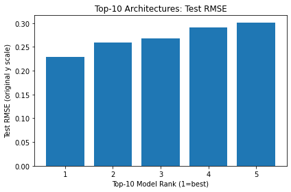

7. Introspection: What worked well?¶

We can check which hyperparameters appear in the winning models. This is not causal inference—just a quick descriptive analysis to support discussion during the lecture.

summary_cols = ["depth","width","activation","batchnorm","dropout","optimizer","batch_size"]
for col in summary_cols:
    display(final_df[col].value_counts())

depth
3    2
1    1
6    1
4    1
Name: count, dtype: int64

width
128    3
32     2
Name: count, dtype: int64

activation
gelu    2
relu    1
elu     1
tanh    1
Name: count, dtype: int64

batchnorm
True     4
False    1
Name: count, dtype: int64

dropout
0.1    2
0.0    2
0.4    1
Name: count, dtype: int64

optimizer
adam       3
rmsprop    2
Name: count, dtype: int64

batch_size
64     2
256    2
128    1
Name: count, dtype: int64

8. Save Artifacts (Optional)¶

We save the top-5 leaderboard and the full random-search table to CSV for later inspection. You can also save models if desired.

os.makedirs("nas_outputs", exist_ok=True)
df.to_csv("nas_outputs/random_search_all_trials.csv", index=False)
final_df.to_csv("nas_outputs/top5_retrained_test_metrics.csv", index=False)
print("Saved:")
print(" - nas_outputs/random_search_all_trials.csv")
print(" - nas_outputs/top5_retrained_test_metrics.csv")

9. Teaching Notes & Extensions¶

Budget vs. space: Increase N_TRIALS or EPOCHS_PER_TRIAL for better results; decrease for speed.
Early stopping: Helps avoid wasted compute on poor configs.
Alternative strategies:
- Successive Halving / Hyperband: Train all a little, keep the best, allocate more epochs iteratively.
- Bayesian Optimization: Use a surrogate model (e.g., Gaussian Process, TPE) to guide sampling.
- Evolutionary Algorithms: Maintain a population of architectures, select/mutate/crossover.
Search space design: Consider residual connections, per-layer activations, weight decay, spectral norm, etc.
Metrics: We use MSE/MAE. For noisy targets, RMSE in original units (back-transformed) is easier to interpret.
Reproducibility: Fix seeds, log versions, save artifacts, record configs for each trial.
Caveat: Random Search is strong but not magic—if the space is huge and the budget is tiny, you may under-sample good regions.

End of notebook.