Course: Deep Learning for Solving and Estimating Dynamic Models in Economics and Finance
Script reference: §4.8 (multi-component losses: the scale problem; inverse-loss weighting; ReLoBRaLo Components 1–3; sensitivity to the temperature )
Notebook role: core
Author: Simon Scheidegger
RUN_MODE = "smoke"  # one of: "smoke", "teaching", "production"
SEED = 0
This notebook accompanies Lecture 05 — Multi-Component Loss Balancing.
Goals:
Understand why multi-component losses at different scales cause problems.
Train a multi-output NN with equal weights and observe failure.
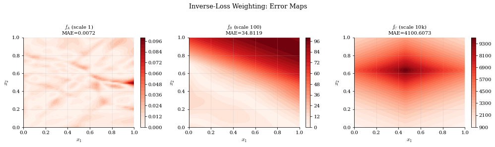
Implement inverse-loss weighting and see partial improvement.
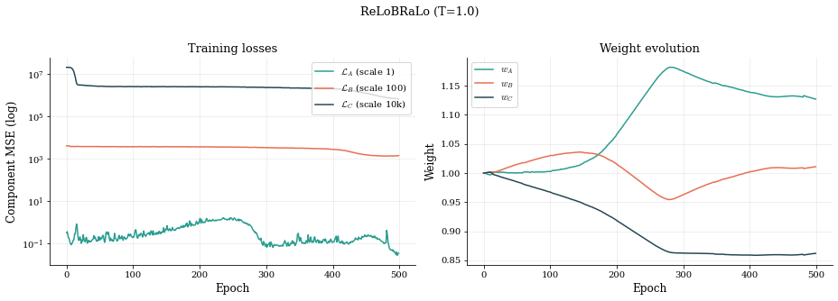
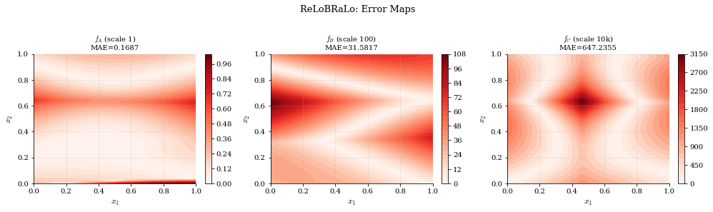
Implement a deterministic classroom version of ReLoBRaLo (Bischof & Kraus, 2025) and achieve balanced learning.
Study sensitivity to the temperature parameter .
Outline
| Section | Topic |
|---|---|
| 1 | Target functions at different scales |
| 2 | Multi-output network |
| 3 | Baseline: equal weighting |
| 4 | Inverse-loss weighting |
| 5 | ReLoBRaLo |
| 6 | Comparison |
| 7 | Sensitivity to |
| 8 | Discussion |
# ----------------------------------------------------------------
# Imports and plot style
# ----------------------------------------------------------------
import numpy as np
import matplotlib.pyplot as plt
from matplotlib import rcParams
from mpl_toolkits.mplot3d import Axes3D  # noqa: F401
import time

import tensorflow as tf
from tensorflow import keras
from tensorflow.keras import layers

# Consistent plot style
rcParams.update({
    "figure.dpi":       120,
    "font.size":        11,
    "axes.titlesize":   13,
    "axes.labelsize":   12,
    "legend.fontsize":  10,
    "xtick.labelsize":  10,
    "ytick.labelsize":  10,
    "font.family":      "serif",
    "mathtext.fontset":  "cm",
    "axes.spines.top":   False,
    "axes.spines.right": False,
    "axes.grid":         True,
    "grid.alpha":        0.25,
})

# Colour palette
C_A     = "#2a9d8f"   # teal (small scale)
C_B     = "#e76f51"   # orange-red (medium scale)
C_C     = "#264653"   # dark blue (large scale)
C_EQUAL = "#6c757d"   # grey
C_INV   = "#e9c46a"   # gold
C_RELO  = "#457b9d"   # steel blue

np.random.seed(42)
tf.random.set_seed(42)

print(f"TensorFlow version: {tf.__version__}")
2026-04-24 12:34:55.990394: E external/local_xla/xla/stream_executor/cuda/cuda_fft.cc:477] Unable to register cuFFT factory: Attempting to register factory for plugin cuFFT when one has already been registered
WARNING: All log messages before absl::InitializeLog() is called are written to STDERR
E0000 00:00:1777026896.028381 308954 cuda_dnn.cc:8310] Unable to register cuDNN factory: Attempting to register factory for plugin cuDNN when one has already been registered
E0000 00:00:1777026896.039160 308954 cuda_blas.cc:1418] Unable to register cuBLAS factory: Attempting to register factory for plugin cuBLAS when one has already been registered
2026-04-24 12:34:56.075776: I tensorflow/core/platform/cpu_feature_guard.cc:210] This TensorFlow binary is optimized to use available CPU instructions in performance-critical operations.
To enable the following instructions: AVX2 FMA, in other operations, rebuild TensorFlow with the appropriate compiler flags.
TensorFlow version: 2.18.0
1. The Multi-Component Loss Problem¶
We approximate three functions simultaneously with a shared-trunk NN. The functions live at vastly different scales:
| Function | Formula | Scale |
|---|---|---|
The composite loss is:
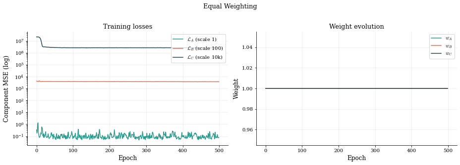
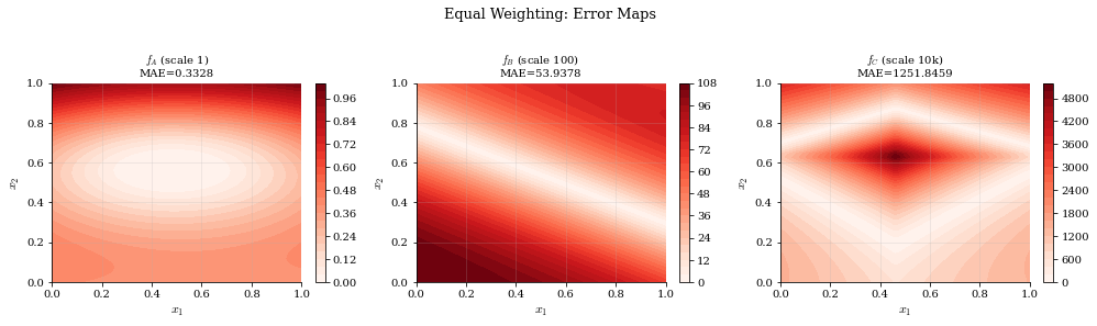
With equal weights (), dominates while is essentially ignored.
# ----------------------------------------------------------------
# Define the three Genz target functions (from Notebook 06)
# ----------------------------------------------------------------

def genz_gaussian(X, c, w):
    """f4: exp(-sum_i c_i^2 * (x_i - w_i)^2)"""
    return np.exp(-np.sum(c**2 * (X - w)**2, axis=1))

def genz_oscillatory(X, c, w):
    """f1: cos(2*pi*w[0] + sum_i c_i * x_i)"""
    return np.cos(2.0 * np.pi * w[0] + X @ c)

def genz_continuous(X, c, w):
    """f5: exp(-sum_i c_i * |x_i - w_i|)"""
    return np.exp(-np.sum(c * np.abs(X - w), axis=1))

# Fixed parameters
d = 2
rng = np.random.RandomState(7)
c_param = rng.uniform(1.0, 3.0, size=d)
w_param = rng.uniform(0.2, 0.8, size=d)

# Multi-scale target functions
def f_A(X): return genz_gaussian(X, c_param, w_param)          # scale ~ 1
def f_B(X): return 100.0 * genz_oscillatory(X, c_param, w_param)  # scale ~ 100
def f_C(X): return 10000.0 * genz_continuous(X, c_param, w_param)  # scale ~ 10000

TARGETS = {"$f_A$ (scale 1)": f_A, "$f_B$ (scale 100)": f_B, "$f_C$ (scale 10k)": f_C}
TARGET_COLORS = [C_A, C_B, C_C]

# Visualise
grid_n = 60
t = np.linspace(0, 1, grid_n)
X1, X2 = np.meshgrid(t, t)
X_grid = np.column_stack([X1.ravel(), X2.ravel()]).astype(np.float32)

fig, axes = plt.subplots(1, 3, figsize=(14, 4),
                         subplot_kw={"projection": "3d"})
for ax, (name, fn), col in zip(axes, TARGETS.items(), TARGET_COLORS):
    Z = fn(X_grid).reshape(grid_n, grid_n)
    ax.plot_surface(X1, X2, Z, cmap="viridis", alpha=0.85,
                    edgecolor="none", rcount=50, ccount=50)
    ax.set_title(name, fontsize=11)
    ax.set_xlabel("$x_1$", fontsize=9)
    ax.set_ylabel("$x_2$", fontsize=9)
    ax.tick_params(labelsize=7)

fig.suptitle("Three target functions at different scales", fontsize=13, y=1.02)
fig.tight_layout()
plt.show()

for name, fn in TARGETS.items():
    vals = fn(X_grid)
    print(f"{name}: range [{vals.min():.2f}, {vals.max():.2f}]")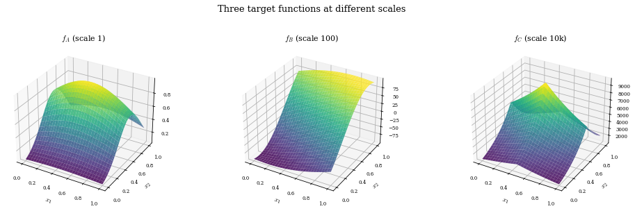
$f_A$ (scale 1): range [0.05, 1.00]
$f_B$ (scale 100): range [-100.00, 100.00]
$f_C$ (scale 10k): range [1062.41, 9762.24]
# ----------------------------------------------------------------
# Generate training and test data
# ----------------------------------------------------------------
n_train = 1000
n_test = 2000

X_train = np.random.uniform(0, 1, size=(n_train, d)).astype(np.float32)
X_test = np.random.uniform(0, 1, size=(n_test, d)).astype(np.float32)

# Targets as arrays: shape (n, 3)
y_train_A = f_A(X_train).astype(np.float32)
y_train_B = f_B(X_train).astype(np.float32)
y_train_C = f_C(X_train).astype(np.float32)

y_test_A = f_A(X_test).astype(np.float32)
y_test_B = f_B(X_test).astype(np.float32)
y_test_C = f_C(X_test).astype(np.float32)

print(f"Training: {n_train} points, Test: {n_test} points")
print(f"MSE scales (train, equal weights):")
print(f"  MSE_A ~ {np.mean(y_train_A**2):.2e}")
print(f"  MSE_B ~ {np.mean(y_train_B**2):.2e}")
print(f"  MSE_C ~ {np.mean(y_train_C**2):.2e}")
Training: 1000 points, Test: 2000 points
MSE scales (train, equal weights):
MSE_A ~ 3.97e-01
MSE_B ~ 4.11e+03
MSE_C ~ 2.12e+07
# ============================================================
# Training-budget switch -- RUN_MODE (set in the run-mode-switch cell) controls all training cells
# ============================================================
# "smoke"      : 200 epochs ~  2 min CPU  (sanity check / CI)
# "teaching"   : 500 epochs ~  6 min CPU  (laptop figures; matches the slide deck)
# "production" : 1500 epochs ~ 18 min CPU  (publication quality)
if RUN_MODE == "smoke":
    EPOCHS_BASE, T_VALUES_SWEEP = 200, [0.1, 1.0]
elif RUN_MODE == "teaching":
    EPOCHS_BASE, T_VALUES_SWEEP = 500, [0.01, 0.1, 1.0, 10.0]
elif RUN_MODE == "production":
    EPOCHS_BASE, T_VALUES_SWEEP = 1500, [0.01, 0.1, 1.0, 10.0]
else:
    raise ValueError(f"Unknown RUN_MODE: {RUN_MODE!r}")
print(f"RUN_MODE = {RUN_MODE}: epochs = {EPOCHS_BASE}, T sweep = {T_VALUES_SWEEP}")
MODE = classroom: epochs = 500, T sweep = [0.01, 0.1, 1.0, 10.0]
# ----------------------------------------------------------------
# Build multi-output Keras model
# ----------------------------------------------------------------

def build_multi_output_model(n_layers=3, n_units=64, activation="relu", lr=1e-3):
    """Shared trunk -> 3 output heads."""
    inp = keras.Input(shape=(d,))
    x = inp
    for _ in range(n_layers):
        x = layers.Dense(n_units, activation=activation)(x)
    # Three output heads
    out_A = layers.Dense(1, name="head_A")(x)
    out_B = layers.Dense(1, name="head_B")(x)
    out_C = layers.Dense(1, name="head_C")(x)
    model = keras.Model(inputs=inp, outputs=[out_A, out_B, out_C])
    return model

# Test
test_model = build_multi_output_model()
test_model.summary()
2026-04-24 12:35:01.559911: E external/local_xla/xla/stream_executor/cuda/cuda_driver.cc:152] failed call to cuInit: INTERNAL: CUDA error: Failed call to cuInit: UNKNOWN ERROR (303)
3. Baseline: Equal Weighting¶
We use a custom training loop so we can log per-component losses and control the weight updates.
# ----------------------------------------------------------------
# Custom training loop with configurable weights
# ----------------------------------------------------------------

def train_multi_output(model, X_tr, y_A, y_B, y_C, X_te, y_te_A, y_te_B, y_te_C,
                       weight_fn, epochs=EPOCHS_BASE, batch_size=64, lr=1e-3,
                       seed=42):
    """
    Train a multi-output model with a custom weight schedule.

    weight_fn: callable(losses, prev_losses, init_losses, prev_weights, epoch)
               -> new_weights (list of 3 floats)
    seed:      reseeds NumPy and TF at function entry so back-to-back
               method comparisons are reproducible regardless of
               cell-execution order.

    The per-batch step is `@tf.function`-compiled so the eager Python
    overhead is paid once per training (not per batch). On CPU this
    typically gives a 5-10x speed-up over the un-jitted version.
    """
    # Re-seed at entry so the per-method shuffle/init are independent of
    # the order in which preceding training cells have consumed the RNG.
    np.random.seed(seed)
    tf.random.set_seed(seed)
    optimizer = keras.optimizers.Adam(learning_rate=lr)
    n = len(X_tr)
    n_batches = max(1, n // batch_size)

    # JIT-compiled per-batch step.  weights enter as a tf.Variable so the
    # graph stays the same when the host code updates them between epochs.
    weights_var = tf.Variable([1.0, 1.0, 1.0], dtype=tf.float32)

    @tf.function
    def train_step(xb, yA, yB, yC):
        with tf.GradientTape() as tape:
            pA, pB, pC = model(xb, training=True)
            lA = tf.reduce_mean(tf.square(yA - pA))
            lB = tf.reduce_mean(tf.square(yB - pB))
            lC = tf.reduce_mean(tf.square(yC - pC))
            total = weights_var[0]*lA + weights_var[1]*lB + weights_var[2]*lC
        grads = tape.gradient(total, model.trainable_variables)
        optimizer.apply_gradients(zip(grads, model.trainable_variables))
        return lA, lB, lC

    # History
    history = {"loss_A": [], "loss_B": [], "loss_C": [],
               "w_A": [], "w_B": [], "w_C": [],
               "test_A": [], "test_B": [], "test_C": []}

    # Initialise
    weights = [1.0, 1.0, 1.0]
    init_losses = None
    prev_losses = None

    # Pre-convert training data once (avoid per-batch tf.constant overhead)
    Xtr_tf = tf.constant(X_tr, dtype=tf.float32)
    yA_tf  = tf.constant(y_A.reshape(-1, 1), dtype=tf.float32)
    yB_tf  = tf.constant(y_B.reshape(-1, 1), dtype=tf.float32)
    yC_tf  = tf.constant(y_C.reshape(-1, 1), dtype=tf.float32)
    Xte_tf = tf.constant(X_te, dtype=tf.float32)

    for epoch in range(epochs):
        weights_var.assign(weights)
        # Shuffle
        idx = np.random.permutation(n)
        epoch_losses = [0.0, 0.0, 0.0]

        for b in range(n_batches):
            sl = idx[b*batch_size : (b+1)*batch_size]
            sl_tf = tf.constant(sl, dtype=tf.int32)
            xb = tf.gather(Xtr_tf, sl_tf)
            yA = tf.gather(yA_tf,  sl_tf)
            yB = tf.gather(yB_tf,  sl_tf)
            yC = tf.gather(yC_tf,  sl_tf)
            lA, lB, lC = train_step(xb, yA, yB, yC)
            epoch_losses[0] += float(lA) / n_batches
            epoch_losses[1] += float(lB) / n_batches
            epoch_losses[2] += float(lC) / n_batches

        # Store initial losses
        if init_losses is None:
            init_losses = list(epoch_losses)
        if prev_losses is None:
            prev_losses = list(epoch_losses)

        # Update weights
        weights = weight_fn(epoch_losses, prev_losses, init_losses, weights, epoch)
        prev_losses = list(epoch_losses)

        # Log
        history["loss_A"].append(epoch_losses[0])
        history["loss_B"].append(epoch_losses[1])
        history["loss_C"].append(epoch_losses[2])
        history["w_A"].append(weights[0])
        history["w_B"].append(weights[1])
        history["w_C"].append(weights[2])

        # Test error (every 10 epochs for speed)
        if epoch % 10 == 0 or epoch == epochs - 1:
            pA_t, pB_t, pC_t = model(Xte_tf, training=False)
            history["test_A"].append(np.abs(pA_t.numpy().flatten() - y_te_A).mean())
            history["test_B"].append(np.abs(pB_t.numpy().flatten() - y_te_B).mean())
            history["test_C"].append(np.abs(pC_t.numpy().flatten() - y_te_C).mean())

    return history


# Equal weighting: weights never change
def equal_weights(losses, prev_losses, init_losses, prev_weights, epoch):
    return [1.0, 1.0, 1.0]


print("Training with equal weights (500 epochs)...")
model_equal = build_multi_output_model()
t0 = time.time()
hist_equal = train_multi_output(
    model_equal, X_train, y_train_A, y_train_B, y_train_C,
    X_test, y_test_A, y_test_B, y_test_C,
    weight_fn=equal_weights, epochs=EPOCHS_BASE
)
print(f"Done in {time.time()-t0:.1f}s")
print(f"Final losses: A={hist_equal['loss_A'][-1]:.4e}, "
      f"B={hist_equal['loss_B'][-1]:.4e}, C={hist_equal['loss_C'][-1]:.4e}")
Training with equal weights (500 epochs)...
Done in 19.3s
Final losses: A=7.6073e-02, B=3.6728e+03, C=2.6013e+06
# ----------------------------------------------------------------
# Visualise equal-weighting results
# ----------------------------------------------------------------

def plot_training_curves(history, title, savename=None):
    """Plot per-component training losses."""
    fig, axes = plt.subplots(1, 2, figsize=(13, 4.5))

    # Loss curves
    ax = axes[0]
    ax.semilogy(history["loss_A"], color=C_A, lw=1.5, label="$\mathcal{L}_A$ (scale 1)")
    ax.semilogy(history["loss_B"], color=C_B, lw=1.5, label="$\mathcal{L}_B$ (scale 100)")
    ax.semilogy(history["loss_C"], color=C_C, lw=1.5, label="$\mathcal{L}_C$ (scale 10k)")
    ax.set_xlabel("Epoch")
    ax.set_ylabel("Component MSE (log)")
    ax.set_title("Training losses")
    ax.legend()

    # Weight evolution
    ax = axes[1]
    ax.plot(history["w_A"], color=C_A, lw=1.5, label="$w_A$")
    ax.plot(history["w_B"], color=C_B, lw=1.5, label="$w_B$")
    ax.plot(history["w_C"], color=C_C, lw=1.5, label="$w_C$")
    ax.set_xlabel("Epoch")
    ax.set_ylabel("Weight")
    ax.set_title("Weight evolution")
    ax.legend()

    fig.suptitle(title, fontsize=13, y=1.02)
    fig.tight_layout()
    if savename is not None:
        fig.savefig(f"../figures/{savename}.pdf", bbox_inches="tight")
        fig.savefig(f"../figures/{savename}.png", dpi=180, bbox_inches="tight")
    plt.show()


def plot_error_heatmaps(model, title, savename=None):
    """Plot per-function |error| heatmaps."""
    pA, pB, pC = model(tf.constant(X_grid), training=False)
    preds = [pA.numpy().flatten(), pB.numpy().flatten(), pC.numpy().flatten()]
    truths = [f_A(X_grid), f_B(X_grid), f_C(X_grid)]
    names = ["$f_A$ (scale 1)", "$f_B$ (scale 100)", "$f_C$ (scale 10k)"]

    fig, axes = plt.subplots(1, 3, figsize=(14, 4))
    for ax, pred, truth, name in zip(axes, preds, truths, names):
        err = np.abs(truth - pred).reshape(grid_n, grid_n)
        im = ax.contourf(X1, X2, err, levels=30, cmap="Reds")
        ax.set_title(f"{name}\nMAE={err.mean():.4f}", fontsize=10)
        ax.set_xlabel("$x_1$")
        ax.set_ylabel("$x_2$")
        plt.colorbar(im, ax=ax, fraction=0.046)

    fig.suptitle(title, fontsize=13, y=1.02)
    fig.tight_layout()
    if savename is not None:
        fig.savefig(f"../figures/{savename}.pdf", bbox_inches="tight")
        fig.savefig(f"../figures/{savename}.png", dpi=180, bbox_inches="tight")
    plt.show()


plot_training_curves(hist_equal, "Equal Weighting", savename="loss_norm_equal_weights")
plot_error_heatmaps(model_equal, "Equal Weighting: Error Maps", savename="loss_norm_equal_errmap")
# ----------------------------------------------------------------
# Inverse-loss weighting
# ----------------------------------------------------------------

# We need a closure to carry the exponential average state
def make_inverse_loss_fn(beta=0.99, eps=1e-8):
    ema = [None, None, None]
    def inverse_loss_weights(losses, prev_losses, init_losses, prev_weights, epoch):
        K = len(losses)
        for i in range(K):
            if ema[i] is None:
                ema[i] = losses[i]
            else:
                ema[i] = beta * ema[i] + (1 - beta) * losses[i]
        raw = [1.0 / (ema[i] + eps) for i in range(K)]
        total = sum(raw)
        return [K * r / total for r in raw]
    return inverse_loss_weights


print(f"Training with inverse-loss weighting ({EPOCHS_BASE} epochs)...")
model_inv = build_multi_output_model()
t0 = time.time()
hist_inv = train_multi_output(
    model_inv, X_train, y_train_A, y_train_B, y_train_C,
    X_test, y_test_A, y_test_B, y_test_C,
    weight_fn=make_inverse_loss_fn(), epochs=EPOCHS_BASE
)
print(f"Done in {time.time()-t0:.1f}s")
print(f"Final losses: A={hist_inv['loss_A'][-1]:.4e}, "
      f"B={hist_inv['loss_B'][-1]:.4e}, C={hist_inv['loss_C'][-1]:.4e}")

plot_training_curves(hist_inv, "Inverse-Loss Weighting")
plot_error_heatmaps(model_inv, "Inverse-Loss Weighting: Error Maps")
Training with inverse-loss weighting (500 epochs)...
Done in 18.3s
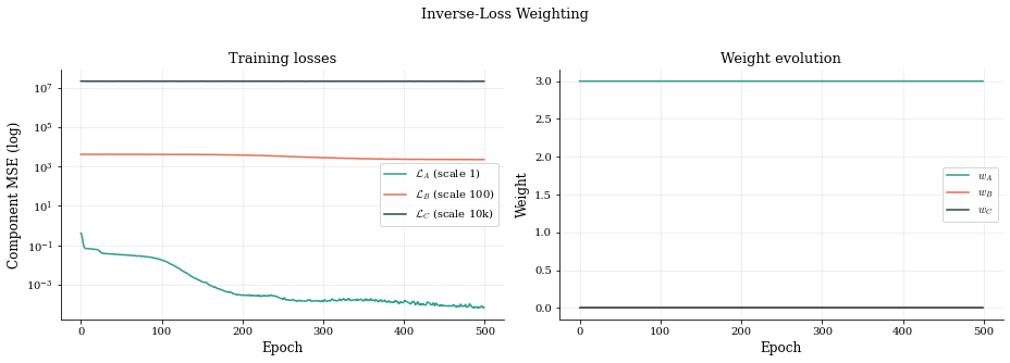
Final losses: A=6.9549e-05, B=2.2504e+03, C=2.1165e+07
5. ReLoBRaLo: Relative Loss Balancing with Random Lookback (deterministic classroom version)¶
Algorithm (Bischof & Kraus, 2025):
At each epoch :
Step-wise weights:
Baseline weights:
Combine:
Hyperparameters: (temperature), (smoothing), (baseline mix in the deterministic classroom version).
# ----------------------------------------------------------------
# ReLoBRaLo implementation
# (adapted from Bischof & Kraus 2025, update_rules.py)
# ----------------------------------------------------------------

def make_relobralo_fn(T=1.0, alpha=0.999, rho=0.999):
    """Create a deterministic ReLoBRaLo-style weight function."""
    def relobralo_weights(losses, prev_losses, init_losses, prev_weights, epoch):
        K = len(losses)
        eps = 1e-12

        # Step-wise relative weights
        ratios = [losses[i] / (prev_losses[i] * T + eps) for i in range(K)]
        exp_ratios = np.exp(ratios - np.max(ratios))  # numerically stable softmax
        w_hat = K * exp_ratios / exp_ratios.sum()

        # Baseline (epoch-0) relative weights
        ratios0 = [losses[i] / (init_losses[i] * T + eps) for i in range(K)]
        exp_ratios0 = np.exp(ratios0 - np.max(ratios0))
        w0_hat = K * exp_ratios0 / exp_ratios0.sum()

        # Combine step-wise and baseline weights with smoothing
        new_weights = [
            rho * alpha * prev_weights[i]
            + (1 - rho) * alpha * w0_hat[i]
            + (1 - alpha) * w_hat[i]
            for i in range(K)
        ]
        return new_weights

    return relobralo_weights


print(f"Training with ReLoBRaLo (T=1.0, {EPOCHS_BASE} epochs)...")
model_relo = build_multi_output_model()
t0 = time.time()
hist_relo = train_multi_output(
    model_relo, X_train, y_train_A, y_train_B, y_train_C,
    X_test, y_test_A, y_test_B, y_test_C,
    weight_fn=make_relobralo_fn(T=1.0), epochs=EPOCHS_BASE
)
print(f"Done in {time.time()-t0:.1f}s")
print(f"Final losses: A={hist_relo['loss_A'][-1]:.4e}, "
      f"B={hist_relo['loss_B'][-1]:.4e}, C={hist_relo['loss_C'][-1]:.4e}")
Training with ReLoBRaLo (T=1.0, 500 epochs)...
Done in 17.5s
Final losses: A=3.5200e-02, B=1.4334e+03, C=6.7153e+05
# ----------------------------------------------------------------
# ReLoBRaLo: weight evolution (key diagnostic plot)
# ----------------------------------------------------------------
plot_training_curves(hist_relo, "ReLoBRaLo (T=1.0)", savename="loss_norm_relobralo_weights")
plot_error_heatmaps(model_relo, "ReLoBRaLo: Error Maps", savename="loss_norm_relobralo_errmap")
# ----------------------------------------------------------------
# Compare all 3 methods
# ----------------------------------------------------------------

def get_test_errors(model):
    pA, pB, pC = model(tf.constant(X_test.astype(np.float32)), training=False)
    err_A = np.abs(pA.numpy().flatten() - y_test_A)
    err_B = np.abs(pB.numpy().flatten() - y_test_B)
    err_C = np.abs(pC.numpy().flatten() - y_test_C)
    return err_A, err_B, err_C

methods = {
    "Equal":       {"model": model_equal, "color": C_EQUAL},
    "Inverse-loss": {"model": model_inv,   "color": C_INV},
    "ReLoBRaLo":   {"model": model_relo,  "color": C_RELO},
}

fn_names = ["$f_A$ (scale 1)", "$f_B$ (scale 100)", "$f_C$ (scale 10k)"]

# Bar chart
fig, axes = plt.subplots(1, 3, figsize=(14, 4.5))

for fn_idx, (fn_name, ax) in enumerate(zip(fn_names, axes)):
    means = []
    maxes = []
    colors = []
    labels = []
    for mname, minfo in methods.items():
        errs = get_test_errors(minfo["model"])
        means.append(errs[fn_idx].mean())
        maxes.append(errs[fn_idx].max())
        colors.append(minfo["color"])
        labels.append(mname)

    x = np.arange(len(labels))
    bars = ax.bar(x, means, color=colors, alpha=0.85, edgecolor="black", linewidth=0.5)
    ax.set_xticks(x)
    ax.set_xticklabels(labels, fontsize=9)
    ax.set_ylabel("Mean |error|")
    ax.set_title(fn_name)
    for bar, val in zip(bars, means):
        ax.text(bar.get_x() + bar.get_width()/2, bar.get_height(),
                f"{val:.4f}", ha="center", va="bottom", fontsize=8)

fig.suptitle("Test Error Comparison: Equal vs Inverse-Loss vs ReLoBRaLo",
             fontsize=13, y=1.02)
fig.tight_layout()
plt.savefig("../figures/loss_norm_method_comparison.pdf", bbox_inches="tight")
plt.savefig("../figures/loss_norm_method_comparison.png", dpi=180, bbox_inches="tight")
plt.show()

# Summary table
print(f"{'Method':<15s}  {'f_A mean':>10s}  {'f_B mean':>10s}  {'f_C mean':>10s}  "
      f"{'f_A max':>10s}  {'f_B max':>10s}  {'f_C max':>10s}")
print("-" * 82)
for mname, minfo in methods.items():
    eA, eB, eC = get_test_errors(minfo["model"])
    print(f"{mname:<15s}  {eA.mean():10.4f}  {eB.mean():10.4f}  {eC.mean():10.4f}  "
          f"{eA.max():10.4f}  {eB.max():10.4f}  {eC.max():10.4f}")
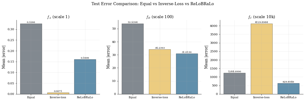
Method             f_A mean    f_B mean    f_C mean     f_A max     f_B max     f_C max
----------------------------------------------------------------------------------
Equal                0.3266     53.9394   1244.0990      1.0187    107.6122   5103.8413
Inverse-loss         0.0071     34.2393   4129.8984      0.0831     98.3490   9739.9639
ReLoBRaLo            0.1606     31.0130    629.8546      0.9705    101.7692   3101.5044
# ----------------------------------------------------------------
# Sensitivity: sweep T in {0.01, 0.1, 1.0, 10.0}
# ----------------------------------------------------------------
T_values = T_VALUES_SWEEP
sensitivity_results = {}

for T_val in T_values:
    print(f"Training ReLoBRaLo with T={T_val}...")
    model_t = build_multi_output_model()
    hist_t = train_multi_output(
        model_t, X_train, y_train_A, y_train_B, y_train_C,
        X_test, y_test_A, y_test_B, y_test_C,
        weight_fn=make_relobralo_fn(T=T_val), epochs=EPOCHS_BASE
    )
    eA, eB, eC = get_test_errors(model_t)
    # Normalised total error (relative to function scale)
    total_rel_err = eA.mean() / 1.0 + eB.mean() / 100.0 + eC.mean() / 10000.0
    sensitivity_results[T_val] = {
        "total_rel_err": total_rel_err,
        "err_A": eA.mean(), "err_B": eB.mean(), "err_C": eC.mean()
    }
    print(f"  Total relative error: {total_rel_err:.4f}")

# Bar chart
fig, ax = plt.subplots(figsize=(8, 4.5))
T_labels = [str(T) for T in T_values]
total_errs = [sensitivity_results[T]["total_rel_err"] for T in T_values]
bar_colors = [C_RELO if err == min(total_errs) else C_EQUAL for err in total_errs]

bars = ax.bar(T_labels, total_errs, color=bar_colors, alpha=0.85,
              edgecolor="black", linewidth=0.5)
ax.set_xlabel("Temperature $T$")
ax.set_ylabel("Total relative error")
ax.set_title("ReLoBRaLo: Sensitivity to Temperature $T$")
for bar, val in zip(bars, total_errs):
    ax.text(bar.get_x() + bar.get_width()/2, bar.get_height(),
            f"{val:.4f}", ha="center", va="bottom", fontsize=9)

fig.tight_layout()
plt.savefig("../figures/loss_norm_T_sensitivity.pdf", bbox_inches="tight")
plt.savefig("../figures/loss_norm_T_sensitivity.png", dpi=180, bbox_inches="tight")
plt.show()

print(f"\n{'T':<6s}  {'Rel. error':>10s}  {'f_A MAE':>10s}  {'f_B MAE':>10s}  {'f_C MAE':>10s}")
print("-" * 52)
for T in T_values:
    r = sensitivity_results[T]
    print(f"{T:<6.2f}  {r['total_rel_err']:10.4f}  {r['err_A']:10.4f}  "
          f"{r['err_B']:10.4f}  {r['err_C']:10.4f}")
Training ReLoBRaLo with T=0.01...
  Total relative error: 0.9764
Training ReLoBRaLo with T=0.1...
  Total relative error: 0.8444
Training ReLoBRaLo with T=1.0...
  Total relative error: 0.8872
Training ReLoBRaLo with T=10.0...
Total relative error: 0.9569
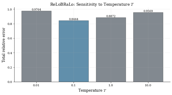
T       Rel. error     f_A MAE     f_B MAE     f_C MAE
----------------------------------------------------
0.01        0.9764      0.3148     53.7564   1240.4087
0.10        0.8444      0.1825     53.7560   1243.6167
1.00        0.8872      0.2174     54.5440   1243.8212
10.00       0.9569      0.2944     53.8152   1243.0726
8. Discussion¶
Key observations¶
Equal weighting fails when loss components differ by more than in scale. The large-scale component dominates the gradient, and the small-scale component is essentially ignored.
Inverse-loss weighting provides a simple fix but can be unstable, especially when losses approach zero.
ReLoBRaLo (Relative Loss Balancing with Random Lookback) provides robust, adaptive balancing by using relative loss changes and a deterministic baseline/history blend that prevents weight drift in this notebook version.
The temperature controls the sharpness of the rebalancing:
: winner-take-all (only one component trained at a time)
: near-equal weights (reverts to the scale problem)
: robust default that works well in most cases
When to use loss balancing in economics¶
PINNs: PDE residual + boundary + initial conditions at different scales
DSGE / DEQNs: Euler equations, budget constraints, and market clearing conditions often have different units and magnitudes
Multi-task learning: Predicting multiple economic variables from shared features (e.g., GDP, inflation, unemployment)
References¶
Bischof & Kraus (2025). Multi-objective loss balancing for physics-informed deep learning. arXiv:2110.09813; published in Computer Methods in Applied Mechanics and Engineering 439:117914, 2025.
Chen, Badrinarayanan, Lee & Rabinovich (2018). GradNorm: Gradient normalization for adaptive loss balancing in deep multitask networks. ICML.
Heydari, Thompson & Mehmood (2019). SoftAdapt: Techniques for adaptive loss weighting of neural networks with multi-part loss functions. arXiv:1912.12355.