Course: Deep Learning for Solving and Estimating Dynamic Models in Economics and Finance
Script reference: §4.3 (random search), §4.5 (Hyperband and successive halving), §4.7 (implementing the search in practice)
Notebook role: core
Author: Simon Scheidegger
RUN_MODE = "smoke"  # one of: "smoke", "teaching", "production"
SEED = 0
Accompanies Lecture 05 — Neural Architecture Search (slides: 04_Neural_Architecture_Search.pdf).
We implement the two key automated-search algorithms from §4 of the lecture script directly, without relying on a hyperparameter-tuning library. The search space and target task are the same as in the slides (Genz Gaussian on , search over depth/width/activation/learning rate), which lets you read off the algorithm logic with no extra abstraction.
Production tooling. Real projects rarely hand-roll the search loop. Established libraries wrap (and parallelize) the same algorithms: KerasTuner, Optuna, Ray Tune, Hyperopt, Ax/BoTorch, NNI, AutoKeras. We mention them here for completeness; the algorithms below are what they all implement underneath.
This is the second of two hands-on NAS examples for Lecture 05:
| Notebook | Method | Testbed |
|---|---|---|
02_NAS_Random_Search_10D.ipynb | Random Search, no external library | 10-D analytical regression |
03_NAS_RandomSearch_Hyperband.ipynb (this notebook) | Random Search + Successive Halving, from scratch | Genz Gaussian on |
Goals
Understand why architecture choice matters for function approximation.
Implement Random Search as a transparent Python loop.
Implement Successive Halving (the building block of Hyperband) as a transparent Python loop.
Compare both against a fixed baseline on the Genz Gaussian test function.
Outline
| Section | Topic |
|---|---|
| 1 | Setup and data generation |
| 2 | Baseline: fixed architecture |
| 3 | Search space and trial helper |
| 4 | Random Search from scratch |
| 5 | Successive Halving from scratch |
| 6 | Comparison and best-model surface |
| 7 | Discussion |
# ----------------------------------------------------------------
# Imports and plot style
# ----------------------------------------------------------------
import numpy as np
import matplotlib.pyplot as plt
from matplotlib import rcParams
from mpl_toolkits.mplot3d import Axes3D  # noqa: F401
import time
import os
import pickle
from pathlib import Path

import tensorflow as tf
from tensorflow import keras
from tensorflow.keras import layers

# Consistent plot style (project convention: font.size = 13)
rcParams.update({
    "figure.dpi":       120,
    "font.size":        13,
    "axes.titlesize":   13,
    "axes.labelsize":   12,
    "legend.fontsize":  10,
    "xtick.labelsize":  10,
    "ytick.labelsize":  10,
    "font.family":      "serif",
    "mathtext.fontset":  "cm",
    "axes.spines.top":   False,
    "axes.spines.right": False,
    "axes.grid":         True,
    "grid.alpha":        0.25,
})

# Colour palette
C_RANDOM  = "#e76f51"   # orange-red, Random Search
C_SHA     = "#2a9d8f"   # teal,       Successive Halving
C_BASE    = "#6c757d"   # grey,       fixed baseline
C_TRUE    = "#457b9d"   # steel blue, ground truth

# Reproducibility (SEED comes from the run-mode-switch cell at the top).
np.random.seed(SEED)
tf.random.set_seed(SEED)

# Cache location for trial records (re-runs short-circuit if present)
CACHE_DIR  = Path("nas_results")
CACHE_DIR.mkdir(exist_ok=True)
CACHE_PATH = CACHE_DIR / "search_records.pkl"

print(f"TensorFlow version: {tf.__version__}")
print(f"Cache file       : {CACHE_PATH}")
2026-04-26 11:55:12.723348: E external/local_xla/xla/stream_executor/cuda/cuda_fft.cc:477] Unable to register cuFFT factory: Attempting to register factory for plugin cuFFT when one has already been registered
WARNING: All log messages before absl::InitializeLog() is called are written to STDERR
E0000 00:00:1777197312.740151  411434 cuda_dnn.cc:8310] Unable to register cuDNN factory: Attempting to register factory for plugin cuDNN when one has already been registered
E0000 00:00:1777197312.745101  411434 cuda_blas.cc:1418] Unable to register cuBLAS factory: Attempting to register factory for plugin cuBLAS when one has already been registered
2026-04-26 11:55:12.770138: I tensorflow/core/platform/cpu_feature_guard.cc:210] This TensorFlow binary is optimized to use available CPU instructions in performance-critical operations.
To enable the following instructions: AVX2 FMA, in other operations, rebuild TensorFlow with the appropriate compiler flags.
TensorFlow version: 2.18.0
Cache file       : nas_results/search_records.pkl
1. The NAS Problem¶
Neural Architecture Search (NAS) aims to find the best network architecture for a given task automatically.
The search space includes:
Number of hidden layers
Number of units per layer
Activation function
Learning rate
We use the Genz Gaussian function on as our test case:
# ----------------------------------------------------------------
# Define Genz Gaussian and generate data
# ----------------------------------------------------------------

def genz_gaussian(X, c, w):
    """f4: exp(-sum_i c_i^2 * (x_i - w_i)^2)"""
    return np.exp(-np.sum(c**2 * (X - w)**2, axis=1))

# Fixed parameters
d = 2
rng = np.random.RandomState(7)
c_param = rng.uniform(1.0, 3.0, size=d)
w_param = rng.uniform(0.2, 0.8, size=d)

# Training and test data
n_train = 1000
n_test = 2000

X_train = np.random.uniform(0, 1, size=(n_train, d)).astype(np.float32)
y_train = genz_gaussian(X_train, c_param, w_param).astype(np.float32)

X_test = np.random.uniform(0, 1, size=(n_test, d)).astype(np.float32)
y_test = genz_gaussian(X_test, c_param, w_param).astype(np.float32)

print(f"d = {d}, c = {c_param}, w = {w_param}")
print(f"Training: {n_train} points, Test: {n_test} points")
print(f"y_train range: [{y_train.min():.3f}, {y_train.max():.3f}]")
d = 2, c = [1.15261658 2.55983758], w = [0.46304554 0.63407911]
Training: 1000 points, Test: 2000 points
y_train range: [0.060, 1.000]
# ----------------------------------------------------------------
# Baseline: fixed 3 x 64 ReLU MLP, ~100 epochs
# ----------------------------------------------------------------

def build_fixed_model(n_layers=3, n_units=64, activation="relu", lr=1e-3):
    """Build a fixed-architecture MLP."""
    model = keras.Sequential()
    model.add(keras.Input(shape=(d,)))
    for _ in range(n_layers):
        model.add(layers.Dense(n_units, activation=activation))
    model.add(layers.Dense(1))
    model.compile(optimizer=keras.optimizers.Adam(learning_rate=lr),
                  loss="mse", metrics=["mae"])
    return model

t0 = time.time()
baseline_model = build_fixed_model()
baseline_history = baseline_model.fit(
    X_train, y_train, epochs=100, batch_size=64, verbose=0,
    validation_data=(X_test, y_test),
)
baseline_time = time.time() - t0

baseline_pred  = baseline_model.predict(X_test, verbose=0).flatten()
baseline_mae   = float(np.abs(baseline_pred - y_test).mean())
baseline_max   = float(np.abs(baseline_pred - y_test).max())
baseline_vloss = float(baseline_history.history["val_loss"][-1])

baseline_record = {
    "config":   {"layers": 3, "units": [64, 64, 64], "activation": "relu", "lr": 1e-3},
    "val_loss": baseline_vloss,
    "mae":      baseline_mae,
    "time":     baseline_time,
    "params":   int(baseline_model.count_params()),
}

print(f"Baseline (3x64 ReLU): MAE = {baseline_mae:.5f}, "
      f"max err = {baseline_max:.5f}, time = {baseline_time:.1f}s")
print(f"Baseline architecture: {baseline_record['params']} parameters")
2026-04-26 11:55:15.981039: E external/local_xla/xla/stream_executor/cuda/cuda_driver.cc:152] failed call to cuInit: INTERNAL: CUDA error: Failed call to cuInit: UNKNOWN ERROR (303)
Baseline (3x64 ReLU): MAE = 0.00556, max err = 0.02280, time = 17.0s
Baseline architecture: 8577 parameters
3. Search space and build_and_train helper¶
Both Random Search and Successive Halving draw architectures from the same search space:
| Hyperparameter | Range |
|---|---|
layers | |
units (per layer) | |
activation | |
lr | log-uniform on |
The trial helper build_and_train(config, epochs) builds the corresponding
keras.Sequential model and trains it for the requested number of epochs with
early stopping on validation loss. It returns the final validation loss and
wall-clock time. This is the only primitive the search algorithms below call.
# ----------------------------------------------------------------
# Search space and trial helper
# ----------------------------------------------------------------

LAYER_OPTIONS = [1, 2, 3, 4, 5]
UNIT_OPTIONS  = [32, 64, 96, 128, 160, 192, 224, 256]
ACT_OPTIONS   = ["relu", "tanh", "swish"]
LR_LOG_LO, LR_LOG_HI = -4.0, -2.0   # log10 bounds for learning rate


def sample_config(rng):
    """Draw one architecture uniformly from the search space."""
    n_layers = int(rng.choice(LAYER_OPTIONS))
    units    = [int(rng.choice(UNIT_OPTIONS)) for _ in range(n_layers)]
    act      = str(rng.choice(ACT_OPTIONS))
    lr       = float(10.0 ** rng.uniform(LR_LOG_LO, LR_LOG_HI))
    return {"layers": n_layers, "units": units, "activation": act, "lr": lr}


def build_model(config):
    """Build a Sequential MLP from a config dict."""
    model = keras.Sequential()
    model.add(keras.Input(shape=(d,)))
    for u in config["units"]:
        model.add(layers.Dense(u, activation=config["activation"]))
    model.add(layers.Dense(1))
    model.compile(
        optimizer=keras.optimizers.Adam(learning_rate=config["lr"]),
        loss="mse",
        metrics=["mae"],
    )
    return model


def build_and_train(config, epochs, X_tr, y_tr, X_val, y_val,
                    batch_size=64, patience=10, verbose=0):
    """Build, fit, and evaluate one trial. Returns a record dict.

    `model.fit` runs Keras' compiled training step (already JIT'd via
    `tf.function` internally), which keeps per-epoch overhead minimal.
    """
    model = build_model(config)
    es = keras.callbacks.EarlyStopping(
        monitor="val_loss", patience=patience,
        restore_best_weights=True, verbose=0,
    )
    t0 = time.time()
    history = model.fit(
        X_tr, y_tr,
        validation_data=(X_val, y_val),
        epochs=epochs, batch_size=batch_size,
        callbacks=[es], verbose=verbose,
    )
    wall = time.time() - t0
    val_loss = float(min(history.history["val_loss"]))
    pred = model.predict(X_val, verbose=0).flatten()
    mae  = float(np.abs(pred - y_val).mean())
    return {
        "config":   config,
        "val_loss": val_loss,
        "mae":      mae,
        "time":     wall,
        "epochs":   len(history.history["val_loss"]),
        "params":   int(model.count_params()),
    }, model


# Quick smoke test
_demo_cfg = sample_config(np.random.default_rng(0))
print("Demo config :", _demo_cfg)
Demo config : {'layers': 5, 'units': [192, 160, 96, 96, 32], 'activation': 'relu', 'lr': 0.0042319495174775335}
# ----------------------------------------------------------------
# Cache: short-circuit on re-run if pickle is present
# ----------------------------------------------------------------
# We pickle a single dict
#     {"random": [...records...], "sha": [...records...], "baseline": {...}}
# to nas_results/search_records.pkl. The plotting cells below read that dict.
# Delete the file to force a fresh sweep.

cache = None
if CACHE_PATH.exists():
    with open(CACHE_PATH, "rb") as f:
        cache = pickle.load(f)
    print(f"Loaded cached records from {CACHE_PATH}")
    print(f"  random : {len(cache['random'])} trials")
    print(f"  sha    : {len(cache['sha'])} trials")
else:
    print(f"No cache at {CACHE_PATH}; the next two cells will run searches.")
No cache at nas_results/search_records.pkl; the next two cells will run searches.
4. Random Search from scratch¶
The loop is six lines of real logic. We sample architectures independently from the search space, train each for a small fixed budget with early stopping, and remember the best.
for i = 1..N:
    cfg     <- sample_config()
    record  <- build_and_train(cfg, epochs=R)
    log(record)
return argmin val_loss over records
Random Search ignores the structure of the response surface, but it is embarrassingly parallel and gives an honest baseline that more sophisticated methods need to beat (Bergstra & Bengio, 2012).
# ----------------------------------------------------------------
# Random Search loop  (budget driven by RUN_MODE; teaching/production = 30 trials x ~50 epochs each)
# ----------------------------------------------------------------
if RUN_MODE == "smoke":
    N_RANDOM_TRIALS, RANDOM_EPOCHS = 8, 12
else:  # "teaching" / "production"
    N_RANDOM_TRIALS, RANDOM_EPOCHS = 30, 50

if cache is not None and "random" in cache:
    random_records = cache["random"]
    print(f"Random Search: using {len(random_records)} cached trials.")
else:
    rng_rs = np.random.default_rng(SEED)
    random_records = []
    t0_rs = time.time()
    for i in range(N_RANDOM_TRIALS):
        cfg = sample_config(rng_rs)
        rec, _ = build_and_train(
            cfg, epochs=RANDOM_EPOCHS,
            X_tr=X_train, y_tr=y_train,
            X_val=X_test, y_val=y_test,
        )
        random_records.append(rec)
        if (i + 1) % 5 == 0 or i == 0:
            best_so_far = min(r["val_loss"] for r in random_records)
            print(f"  trial {i+1:>2d}/{N_RANDOM_TRIALS}: "
                  f"val_loss={rec['val_loss']:.2e}  "
                  f"best={best_so_far:.2e}  "
                  f"({rec['epochs']} epochs, {rec['time']:.1f}s)")
    random_total_time = time.time() - t0_rs
    print(f"Random Search done in {random_total_time:.1f}s "
          f"({len(random_records)} trials)")

best_random = min(random_records, key=lambda r: r["val_loss"])
print(f"\nBest Random Search config : {best_random['config']}")
print(f"  val_loss = {best_random['val_loss']:.3e}, MAE = {best_random['mae']:.5f}")
trial 1/30: val_loss=4.43e-02 best=4.43e-02 (14 epochs, 2.6s)
trial 5/30: val_loss=2.68e-04 best=3.14e-06 (50 epochs, 7.4s)
trial 10/30: val_loss=4.16e-04 best=3.14e-06 (50 epochs, 7.9s)
trial 15/30: val_loss=6.08e-04 best=3.14e-06 (50 epochs, 8.1s)
trial 20/30: val_loss=3.34e-03 best=3.14e-06 (34 epochs, 7.3s)
trial 25/30: val_loss=2.80e-02 best=3.14e-06 (50 epochs, 6.0s)
  trial 30/30: val_loss=8.92e-06  best=2.38e-06  (50 epochs, 9.1s)
Random Search done in 222.0s (30 trials)

Best Random Search config : {'layers': 4, 'units': [192, 192, 128, 192], 'activation': 'relu', 'lr': 0.0010048229603696426}
  val_loss = 2.385e-06, MAE = 0.00120
5. Successive Halving from scratch¶
Successive Halving (SHA) is the inner loop of Hyperband (Li et al., 2018). The idea: cheap configurations should be killed early, expensive ones promoted.
We use initial random configs and a halving rate , giving three rounds and a 1-of-27 winner:
| Round | Configs alive | Epoch budget per config |
|---|---|---|
| 0 | 27 | |
| 1 | 9 | |
| 2 | 3 | |
| 3 | 1 | (final winner) |
Each round, we train every surviving config for r_k epochs, sort by
validation loss, and keep the top . The total epoch budget is roughly
matched to Random Search (
epoch-trials, vs for Random Search), but SHA spends most
of its compute on the promising tail.
# ----------------------------------------------------------------
# Successive Halving (SHA) loop
# ----------------------------------------------------------------
ETA = 3                # halving rate
if RUN_MODE == "smoke":
    N0_SHA, R0, N_ROUNDS = 9, 4, 2     # 9@4 -> 3@12 -> winner
else:  # "teaching" / "production"
    N0_SHA, R0, N_ROUNDS = 27, 8, 3    # 27@8 -> 9@24 -> 3@72 -> winner

if cache is not None and "sha" in cache:
    sha_records = cache["sha"]
    print(f"SHA: using {len(sha_records)} cached trials.")
else:
    rng_sha = np.random.default_rng(SEED + 1)
    # Round 0: sample n0 configs and train each for R0 epochs
    survivors = [sample_config(rng_sha) for _ in range(N0_SHA)]
    sha_records = []
    t0_sha = time.time()
    for k in range(N_ROUNDS):
        epochs_k = R0 * (ETA ** k)
        print(f"Round {k}: {len(survivors)} configs x {epochs_k} epochs")
        round_records = []
        for j, cfg in enumerate(survivors):
            rec, _ = build_and_train(
                cfg, epochs=epochs_k,
                X_tr=X_train, y_tr=y_train,
                X_val=X_test, y_val=y_test,
            )
            rec["round"] = k
            round_records.append(rec)
            sha_records.append(rec)
        # Promote top 1/eta
        round_records.sort(key=lambda r: r["val_loss"])
        n_keep = max(1, len(round_records) // ETA)
        survivors = [r["config"] for r in round_records[:n_keep]]
        print(f"  best this round : val_loss={round_records[0]['val_loss']:.2e}")
        print(f"  promoting top {n_keep} -> next round")
    sha_total_time = time.time() - t0_sha
    print(f"SHA done in {sha_total_time:.1f}s "
          f"(total trials evaluated: {len(sha_records)})")

best_sha = min(sha_records, key=lambda r: r["val_loss"])
print(f"\nBest SHA config : {best_sha['config']}")
print(f"  val_loss = {best_sha['val_loss']:.3e}, MAE = {best_sha['mae']:.5f}")
Round 0: 27 configs x 8 epochs
  best this round : val_loss=5.14e-04
  promoting top 9 -> next round
Round 1: 9 configs x 24 epochs
  best this round : val_loss=2.99e-06
  promoting top 3 -> next round
Round 2: 3 configs x 72 epochs
  best this round : val_loss=1.75e-06
  promoting top 1 -> next round
SHA done in 135.7s (total trials evaluated: 39)

Best SHA config : {'layers': 5, 'units': [256, 256, 224, 192, 128], 'activation': 'relu', 'lr': 0.0010026588780510212}
  val_loss = 1.753e-06, MAE = 0.00100
# ----------------------------------------------------------------
# Persist trial records so re-runs short-circuit
# ----------------------------------------------------------------
if cache is None:
    cache = {
        "random":   random_records,
        "sha":      sha_records,
        "baseline": baseline_record,
    }
    with open(CACHE_PATH, "wb") as f:
        pickle.dump(cache, f)
    print(f"Wrote {CACHE_PATH} ({len(random_records)} RS + "
          f"{len(sha_records)} SHA records).")
else:
    print(f"Cache already on disk at {CACHE_PATH}; nothing to write.")
Wrote nas_results/search_records.pkl (30 RS + 39 SHA records).
6. Comparison and best-model surface¶
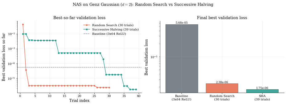
We plot the best-so-far validation loss against trial index for each
algorithm. The fixed baseline appears as a constant horizontal line. This is
the figure consumed by the slides as nas_search_results.pdf.
# ----------------------------------------------------------------
# Figure 1: best-so-far comparison (saved as nas_search_results.{pdf,png})
# ----------------------------------------------------------------

def best_so_far(records):
    """Cumulative minimum of val_loss along the trial sequence."""
    out, m = [], np.inf
    for r in records:
        m = min(m, r["val_loss"])
        out.append(m)
    return np.asarray(out)

rs_curve  = best_so_far(random_records)
sha_curve = best_so_far(sha_records)

fig, axes = plt.subplots(1, 2, figsize=(13, 4.6))

# (a) Best-so-far validation loss vs trial index
ax = axes[0]
ax.plot(np.arange(1, len(rs_curve) + 1),  rs_curve,  marker="o", ms=4,
        color=C_RANDOM, label=f"Random Search ({len(rs_curve)} trials)")
ax.plot(np.arange(1, len(sha_curve) + 1), sha_curve, marker="s", ms=4,
        color=C_SHA,    label=f"Successive Halving ({len(sha_curve)} trials)")
ax.axhline(baseline_record["val_loss"], color=C_BASE, ls="--", lw=1.2,
           label=f"Baseline (3x64 ReLU)")
ax.set_yscale("log")
ax.set_xlabel("Trial index")
ax.set_ylabel("Best validation loss so far")
ax.set_title("Best-so-far validation loss")
ax.legend(loc="upper right", frameon=False)

# (b) Final best val_loss bar chart
ax = axes[1]
labels = ["Baseline\n(3x64 ReLU)",
          f"Random Search\n({len(random_records)} trials)",
          f"SHA\n({len(sha_records)} trials)"]
vals   = [baseline_record["val_loss"],
          float(rs_curve[-1]),
          float(sha_curve[-1])]
colors = [C_BASE, C_RANDOM, C_SHA]
bars = ax.bar(labels, vals, color=colors, alpha=0.9,
              edgecolor="black", linewidth=0.5)
ax.set_yscale("log")
ax.set_ylabel("Best validation loss")
ax.set_title("Final best validation loss")
for bar, v in zip(bars, vals):
    ax.text(bar.get_x() + bar.get_width() / 2, bar.get_height(),
            f"{v:.2e}", ha="center", va="bottom", fontsize=9)

fig.suptitle("NAS on Genz Gaussian ($d=2$): Random Search vs Successive Halving",
             fontsize=13, y=1.02)
fig.tight_layout()

fig_path_pdf = "../figures/nas_search_results.pdf"
fig_path_png = "../figures/nas_search_results.png"
plt.savefig(fig_path_pdf, bbox_inches="tight")
plt.savefig(fig_path_png, dpi=180, bbox_inches="tight")
plt.show()

# Print a small summary table
print(f"\n{'Method':<22s}  {'Best val_loss':>14s}  {'Best MAE':>10s}")
print("-" * 50)
print(f"{'Baseline (3x64 ReLU)':<22s}  {baseline_record['val_loss']:14.3e}  "
      f"{baseline_record['mae']:10.5f}")
print(f"{'Random Search (30)':<22s}  {best_random['val_loss']:14.3e}  "
      f"{best_random['mae']:10.5f}")
print(f"{'SHA (27/9/3/1)':<22s}  {best_sha['val_loss']:14.3e}  "
      f"{best_sha['mae']:10.5f}")
Method                   Best val_loss    Best MAE
--------------------------------------------------
Baseline (3x64 ReLU)         5.676e-05     0.00556
Random Search (30)           2.385e-06     0.00120
SHA (27/9/3/1)               1.753e-06     0.00100
# ----------------------------------------------------------------
# Figure 2: best-model surface (saved as nas_best_surface.{pdf,png})
# ----------------------------------------------------------------
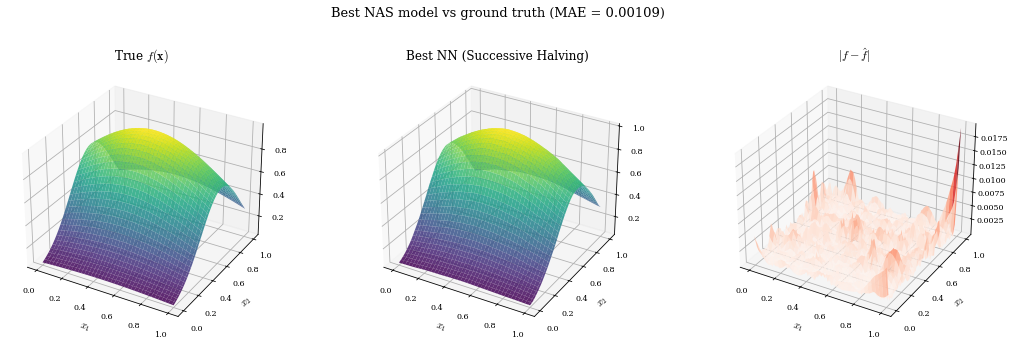
# We retrain the best config (across both searches) for a generous epoch
# budget so the surface plot reflects the architecture, not the search
# transient.

best_overall = min([best_random, best_sha], key=lambda r: r["val_loss"])
best_method  = "Random Search" if best_overall is best_random else "Successive Halving"
print(f"Best overall method : {best_method}")
print(f"Best config         : {best_overall['config']}")
print(f"  val_loss = {best_overall['val_loss']:.3e}, MAE = {best_overall['mae']:.5f}")

# Re-fit the winner with a longer budget for a clean surface
final_rec, final_model = build_and_train(
    best_overall["config"], epochs=300,
    X_tr=X_train, y_tr=y_train,
    X_val=X_test, y_val=y_test,
    patience=30,
)
print(f"Re-fit MAE = {final_rec['mae']:.5f} after {final_rec['epochs']} epochs")

# Build evaluation grid
grid_n = 80
t_grid = np.linspace(0, 1, grid_n)
X1, X2 = np.meshgrid(t_grid, t_grid)
X_grid = np.column_stack([X1.ravel(), X2.ravel()]).astype(np.float32)

Z_true = genz_gaussian(X_grid, c_param, w_param).reshape(grid_n, grid_n)
Z_pred = final_model.predict(X_grid, verbose=0).reshape(grid_n, grid_n)
Z_err  = np.abs(Z_true - Z_pred)

fig, axes = plt.subplots(1, 3, figsize=(15, 4.6),
                         subplot_kw={"projection": "3d"})

axes[0].plot_surface(X1, X2, Z_true, cmap="viridis", alpha=0.85,
                     edgecolor="none", rcount=60, ccount=60)
axes[0].set_title(r"True $f(\mathbf{x})$", fontsize=12)

axes[1].plot_surface(X1, X2, Z_pred, cmap="viridis", alpha=0.85,
                     edgecolor="none", rcount=60, ccount=60)
axes[1].set_title(f"Best NN ({best_method})", fontsize=12)

axes[2].plot_surface(X1, X2, Z_err, cmap="Reds", alpha=0.85,
                     edgecolor="none", rcount=60, ccount=60)
axes[2].set_title(r"$|f - \hat f|$", fontsize=12)

for ax in axes:
    ax.set_xlabel(r"$x_1$", fontsize=10)
    ax.set_ylabel(r"$x_2$", fontsize=10)
    ax.tick_params(labelsize=8)

fig.suptitle(f"Best NAS model vs ground truth (MAE = {Z_err.mean():.5f})",
             fontsize=13, y=1.02)
fig.tight_layout()

surf_pdf = "../figures/nas_best_surface.pdf"
surf_png = "../figures/nas_best_surface.png"
plt.savefig(surf_pdf, bbox_inches="tight")
plt.savefig(surf_png, dpi=180, bbox_inches="tight")
plt.show()
Best overall method : Successive Halving
Best config         : {'layers': 5, 'units': [256, 256, 224, 192, 128], 'activation': 'relu', 'lr': 0.0010026588780510212}
  val_loss = 1.753e-06, MAE = 0.00100
Re-fit MAE = 0.00106 after 75 epochs
7. Discussion¶
Key observations¶
Both automated methods beat the fixed baseline. Even with only 30 trials, Random Search finds an architecture better than our intuition-driven ReLU choice (Bergstra & Bengio, 2012).
Random Search is a surprisingly strong baseline. Sampling independently across all hyperparameters covers the important dimensions well, especially when only a few axes matter (here, learning rate and width).
Successive Halving spends compute where it pays off. By killing poorly-initialized configs after epochs, SHA reallocates the budget to the long tail of survivors. Hyperband (Li et al., 2018) wraps SHA in an outer loop over different initial pairs to hedge against the early-stopping bias.
Bayesian Optimisation (not implemented here) typically matches or slightly beats Random Search on smooth, low-dimensional response surfaces, at the cost of a sequential bottleneck. We cover the GP + Expected Improvement machinery in Day 7 (Surrogates, GPs, and Bayesian Estimation).
When does NAS matter in economics?¶
Surrogate models. When replacing expensive simulations (climate models, agent-based models) with neural networks, architecture choice directly determines approximation quality.
Policy function approximation. In deep equilibrium nets (Lecture 03), the NN approximates policy/value functions. NAS can automate the architecture selection that is usually done by hand.
Diminishing returns. For simple functions (), 30 random trials is usually enough. For high-dimensional problems, the budget should scale with input dimension, and SHA / Hyperband become essential to keep wall-clock time tractable.
Production tooling (footnote)¶
The from-scratch loops above are pedagogical. In practice you would reach for:
KerasTuner -- the most natural fit for TF/Keras workflows
Optuna -- framework-agnostic, define-by-run search spaces
Ray Tune -- distributed trials, integrates with PBT and HEBO
Hyperopt -- TPE algorithm out of the box
Ax / BoTorch -- modern Bayesian optimization on PyTorch
NNI, AutoKeras -- broader AutoML pipelines
Every one of these libraries implements the algorithms above (and a few more) under the hood. Knowing the algorithm makes it easier to read their docs and to debug when a search underperforms.
References¶
Bergstra, J., & Bengio, Y. (2012). Random search for hyper-parameter optimization. JMLR 13, 281-305.
Li, L., Jamieson, K., DeSalvo, G., Rostamizadeh, A., & Talwalkar, A. (2018). Hyperband: A novel bandit-based approach to hyperparameter optimization. JMLR 18(185), 1-52.
Garnett, R. (2023). Bayesian optimization. Cambridge University Press.
Snoek, J., Larochelle, H., & Adams, R. P. (2012). Practical Bayesian optimization of machine learning algorithms. NeurIPS.