Lecture 09, Notebook 10: Young’s non-stochastic simulation by example

Course: Deep Learning for Solving and Estimating Dynamic Models in Economics and Finance
Script reference: §6.3 (Young’s non-stochastic simulation)
Notebook role: core
Author: Simon Scheidegger

RUN_MODE = "smoke"  # one of: "smoke", "teaching", "production"
SEED = 0

Young’s (2010) Method to Simulate a Cross-Section¶

Python implementation based on Julien Pascal’s notebook

Reference: Young, E.R. (2010). “Solving the incomplete markets model with aggregate uncertainty using the Krusell–Smith algorithm and non-stochastic simulations.” Journal of Economic Dynamics and Control, 34(1), 36–41.

Overview¶

Solving economic models with heterogeneous agents involves two key steps:

Finding the optimal response of individuals (policy functions)
Simulating the model to track how the cross-sectional distribution evolves

Young’s (2010) method addresses step 2: instead of simulating a panel of agents (Monte Carlo), we simulate the distribution directly on a fixed grid — deterministically, with no sampling noise.

Pedagogical role in Day 4¶

This notebook isolates the Young update operator itself. The companion notebook 11_Continuum_of_Agents_DEQN.ipynb then uses the same histogram logic inside the larger Appendix A.5 DEQN teaching model. So the move from this notebook (10) to notebook 11 is a change in the surrounding equilibrium architecture, not a change in the distribution update method.

This notebook demonstrates:¶

The core mass redistribution algorithm
Approximating a single mass point
Approximating a multi-point distribution (truncated normal)
Mean preservation property
Comparison with panel-based simulation (Monte Carlo)
Convergence analysis: how many agents does the panel approach need?
The conceptual bridge to the DEQN implementation in notebook 11
Reproducing the script’s hand-worked 4-point Young update (Chapter 6, §6.3)

Run mode. This notebook uses small, fixed example sizes by design: the kit-mandated RUN_MODE constant is present only for consistency across the kit, but the toy grids and panels below do not depend on it. SEED reseeds the Monte-Carlo comparisons.

import numpy as np
import matplotlib.pyplot as plt
from scipy.stats import truncnorm

# Plotting style
plt.rcParams.update({
    'figure.figsize': (10, 6),
    'font.size': 13,
    'axes.grid': True,
    'grid.alpha': 0.3,
    'axes.spines.top': False,
    'axes.spines.right': False,
})

1. The Method¶

Core idea¶

Choose a fixed grid $[w_1, w_2, \ldots, w_N]$ and represent the distribution as a histogram — a vector of masses at each grid point.

When a value $w$ falls between grid points $w_n$ and $w_{n+1}$ , split its mass using linear interpolation:

p = 1 - \frac{w - w_n}{w_{n+1} - w_n}

(1)

Mass assigned to $w_n$ : $m \times p$
Mass assigned to $w_{n+1}$ : $m \times (1 - p)$

Key property: This preserves the mean exactly (when the grid is wide enough).

2. Helper Functions¶

def closest_index(grid, x):
    """Find the index of the closest grid point to x."""
    idx = np.searchsorted(grid, x)
    # Handle boundaries
    if idx == 0:
        return 0
    if idx == len(grid):
        return len(grid) - 1
    # Compare distances to neighbors
    if abs(grid[idx] - x) < abs(grid[idx - 1] - x):
        return idx
    else:
        return idx - 1


def redistribute_mass_single(w, mass, grid):
    """
    Redistribute a single mass point onto the grid using Young's method.
    
    Parameters
    ----------
    w : float
        True value of the mass point.
    mass : float  
        Amount of mass at this point.
    grid : array
        The fixed grid of points.
    
    Returns
    -------
    hw_grid : array
        Histogram of mass on the grid.
    """
    n = len(grid)
    hw_grid = np.zeros(n)
    w_min, w_max = grid[0], grid[-1]
    
    # Find closest grid point
    idx_proj = closest_index(grid, w)
    w_proj = grid[idx_proj]
    
    # Determine bracketing indices
    if w >= w_proj:
        idx_below = idx_proj
        idx_above = idx_proj + 1
    else:
        idx_below = idx_proj - 1
        idx_above = idx_proj
    
    # Boundary cases
    idx_below = np.clip(idx_below, 0, n - 1)
    idx_above = np.clip(idx_above, 0, n - 1)
    
    # Compute interpolation weight p
    if w <= w_min:
        p = 1.0  # all mass to first grid point
    elif w >= w_max:
        p = 0.0  # all mass to last grid point
    else:
        denom = grid[idx_above] - grid[idx_below]
        if denom == 0:
            p = 1.0
        else:
            p = 1.0 - (w - grid[idx_below]) / denom
            p = np.clip(p, 0.0, 1.0)
    
    # Spread the mass
    hw_grid[idx_below] += p * mass
    hw_grid[idx_above] += (1.0 - p) * mass
    
    return hw_grid


def redistribute_distribution(w_true, mass_true, grid):
    """
    Redistribute a multi-point distribution onto a grid using Young's method.
    
    Parameters
    ----------
    w_true : array
        Locations of the true mass points.
    mass_true : array
        Mass at each true point (should sum to 1).
    grid : array
        The fixed grid of points.
    
    Returns
    -------
    hw_grid : array
        Histogram of mass on the grid.
    """
    n = len(grid)
    hw_grid = np.zeros(n)
    
    for w, mass in zip(w_true, mass_true):
        hw_grid += redistribute_mass_single(w, mass, grid)
    
    return hw_grid


def weighted_mean(values, weights):
    """Compute the weighted mean."""
    return np.average(values, weights=weights)


def weighted_var(values, weights):
    """Compute the weighted variance."""
    mu = weighted_mean(values, weights)
    return np.average((values - mu) ** 2, weights=weights)


def weighted_quantile(values, weights, q):
    """Compute the weighted quantile."""
    sorted_idx = np.argsort(values)
    sorted_values = values[sorted_idx]
    sorted_weights = weights[sorted_idx]
    cum_weights = np.cumsum(sorted_weights)
    cum_weights /= cum_weights[-1]  # normalize
    return np.interp(q, cum_weights, sorted_values)

3. Example 1: Single Mass Point¶

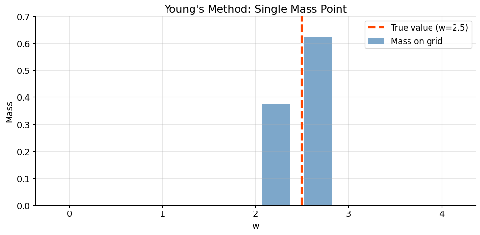
Consider a single mass point at $w = 2.5$ with mass $m = 1.0$ . The grid has 10 points equally spaced on $[0, 4]$ .

Since $w = 2.5$ is not a grid point, Young’s method splits the mass between the two nearest grid points.

# True value
w = 2.5
mass = 1.0

# Approximation grid
n_grid = 10
w_grid = np.linspace(0.0, 4.0, n_grid)
print(f"Grid points: {w_grid}")
print(f"Grid spacing: {w_grid[1] - w_grid[0]:.4f}")

# Redistribute
hw_grid = redistribute_mass_single(w, mass, w_grid)

# Plot
fig, ax = plt.subplots(figsize=(10, 5))
ax.bar(w_grid, hw_grid, width=0.3, alpha=0.7, color='steelblue', label='Mass on grid')
ax.axvline(w, color='orangered', linewidth=3, linestyle='--', label=f'True value (w={w})')
ax.set_xlabel('w')
ax.set_ylabel('Mass')
ax.set_title('Young\'s Method: Single Mass Point')
ax.legend(fontsize=12)
ax.set_ylim(0, 0.7)
plt.tight_layout()
plt.show()

# Check mean preservation
true_mean = w
approx_mean = weighted_mean(w_grid, hw_grid)
print(f"True mean:        {true_mean}")
print(f"Approximate mean: {approx_mean}")
print(f"Difference:       {abs(true_mean - approx_mean):.2e}")

Grid points: [0.         0.44444444 0.88888889 1.33333333 1.77777778 2.22222222
 2.66666667 3.11111111 3.55555556 4.        ]
Grid spacing: 0.4444

True mean:        2.5
Approximate mean: 2.5
Difference:       0.00e+00

What happened?¶

The true value $w = 2.5$ falls between grid points $w_5 \approx 2.22$ and $w_6 \approx 2.67$ . The mass is split proportionally:

p = 1 - \frac{2.5 - 2.22}{2.67 - 2.22} \approx 0.375

(2)

So ~37.5% of the mass goes to $w_5$ and ~62.5% goes to $w_6$ . The mean is preserved exactly.

4. Example 2: Multi-Point Distribution (Truncated Normal)¶

Now consider a more realistic case: the true distribution is a truncated normal on $[1, 3]$ with mean 2. We evaluate it at 10 equally spaced points, then project it onto a different (coarser or finer) grid.

# True distribution: truncated normal on [1, 3] centered at 2
# (Matching Method.pdf: Julia's Normal(2.0) has sigma=1.0 by default)
N_true = 10
w_true_lb, w_true_ub = 1.0, 3.0
mu_true = (w_true_lb + w_true_ub) / 2  # = 2.0
sigma_true = 1.0  # Julia default: Normal(mu) has sigma=1

# scipy's truncnorm uses standardized bounds
a_tn = (w_true_lb - mu_true) / sigma_true
b_tn = (w_true_ub - mu_true) / sigma_true
dist = truncnorm(a_tn, b_tn, loc=mu_true, scale=sigma_true)

# Evaluate at N_true equally spaced points
w_true = np.linspace(w_true_lb, w_true_ub, N_true)
mass_true = dist.pdf(w_true)
mass_true /= mass_true.sum()  # normalize to sum to 1

# Plot the true distribution
fig, ax = plt.subplots(figsize=(10, 5))
ax.bar(w_true, mass_true, width=0.15, alpha=0.8, color='steelblue', label='True distribution')
ax.set_xlabel('w')
ax.set_ylabel('Mass')
ax.set_title('True Distribution: Truncated Normal on [1, 3]')
ax.legend(fontsize=12)
plt.tight_layout()
plt.show()

print(f"True mean:     {weighted_mean(w_true, mass_true):.4f}")
print(f"True median:   {weighted_quantile(w_true, mass_true, 0.5):.4f}")
print(f"True variance: {weighted_var(w_true, mass_true):.4f}")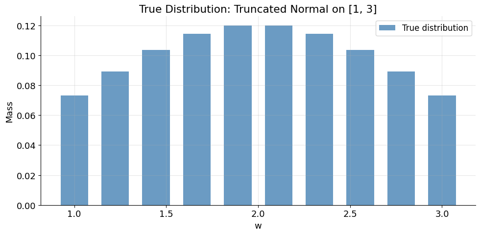

True mean:     2.0000
True median:   1.8889
True variance: 0.3465

# Approximation grid: 10 points on [0, 4] (same as Method.pdf)
n_approx = 10
w_grid = np.linspace(0.0, 4.0, n_approx)

# Redistribute the true distribution onto the approximation grid
hw_grid = redistribute_distribution(w_true, mass_true, w_grid)

# Plot comparison
fig, axes = plt.subplots(1, 2, figsize=(14, 5))

# Left: true distribution
axes[0].bar(w_true, mass_true, width=0.15, alpha=0.8, color='steelblue')
axes[0].set_xlabel('w')
axes[0].set_ylabel('Mass')
axes[0].set_title('True Distribution')
axes[0].set_xlim(-0.2, 4.2)
axes[0].set_ylim(0, max(mass_true) * 1.2)

# Right: Young's approximation
axes[1].bar(w_grid, hw_grid, width=0.3, alpha=0.7, color='orangered', label="Young's approx.")
axes[1].bar(w_true, mass_true, width=0.12, alpha=0.5, color='steelblue', label='True')
axes[1].set_xlabel('w')
axes[1].set_ylabel('Mass')
axes[1].set_title("Young's Approximation on Grid")
axes[1].set_xlim(-0.2, 4.2)
axes[1].set_ylim(0, max(max(mass_true), max(hw_grid)) * 1.2)
axes[1].legend(fontsize=11)

plt.suptitle(f'True grid: {N_true} points on [1,3]  →  Approx. grid: {n_approx} points on [0,4]',
             fontsize=13, y=1.02)
plt.tight_layout()
plt.show()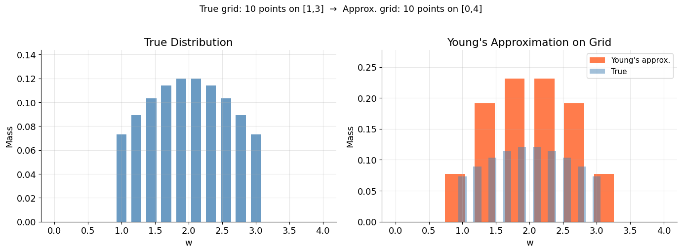

# Compare moments
true_mean = weighted_mean(w_true, mass_true)
approx_mean = weighted_mean(w_grid, hw_grid)

true_median = weighted_quantile(w_true, mass_true, 0.5)
approx_median = weighted_quantile(w_grid, hw_grid, 0.5)

true_var = weighted_var(w_true, mass_true)
approx_var = weighted_var(w_grid, hw_grid)

print("Moment Comparison: Young's Method vs. True Distribution")
print("=" * 55)
print(f"{'':20s} {'True':>12s} {'Approx':>12s} {'Error':>12s}")
print("-" * 55)
print(f"{'Mean':20s} {true_mean:12.4f} {approx_mean:12.4f} {abs(true_mean-approx_mean):12.2e}")
print(f"{'Median':20s} {true_median:12.4f} {approx_median:12.4f} {abs(true_median-approx_median):12.2e}")
print(f"{'Variance':20s} {true_var:12.4f} {approx_var:12.4f} {abs(true_var-approx_var):12.2e}")
print("=" * 55)
print("\n→ Mean is preserved exactly; higher moments are approximated.")

Moment Comparison: Young's Method vs. True Distribution
=======================================================
                             True       Approx        Error
-------------------------------------------------------
Mean                       2.0000       2.0000     0.00e+00
Median                     1.8889       1.7778     1.11e-01
Variance                   0.3465       0.3836     3.70e-02
=======================================================

→ Mean is preserved exactly; higher moments are approximated.

The mean is always preserved, but higher moments (variance, median) improve with finer grids.

grid_sizes = [5, 10, 20, 50, 100, 200, 500]
mean_errors = []
var_errors = []
median_errors = []

for ng in grid_sizes:
    g = np.linspace(0.0, 4.0, ng)
    h = redistribute_distribution(w_true, mass_true, g)
    
    mean_errors.append(abs(weighted_mean(g, h) - true_mean))
    var_errors.append(abs(weighted_var(g, h) - true_var))
    median_errors.append(abs(weighted_quantile(g, h, 0.5) - true_median))

fig, ax = plt.subplots(figsize=(10, 6))
ax.semilogy(grid_sizes, mean_errors, 'o-', linewidth=2, markersize=8, label='Mean error')
ax.semilogy(grid_sizes, var_errors, 's-', linewidth=2, markersize=8, label='Variance error')
ax.semilogy(grid_sizes, median_errors, '^-', linewidth=2, markersize=8, label='Median error')
ax.set_xlabel('Number of grid points')
ax.set_ylabel('Absolute error')
ax.set_title("Young's Method: Approximation Error vs. Grid Size")
ax.legend(fontsize=12)
ax.set_ylim(bottom=1e-16)
plt.tight_layout()
plt.show()

print("→ Mean error stays at machine precision regardless of grid size.")
print("→ Variance and median errors decrease with finer grids.")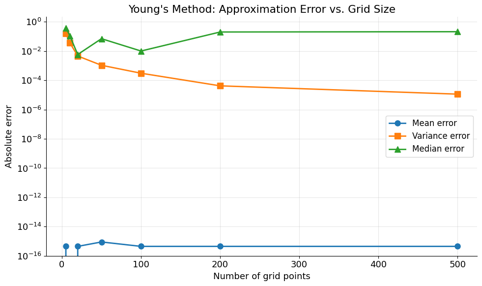

→ Mean error stays at machine precision regardless of grid size.
→ Variance and median errors decrease with finer grids.

6. Panel Simulation (Monte Carlo Alternative)¶

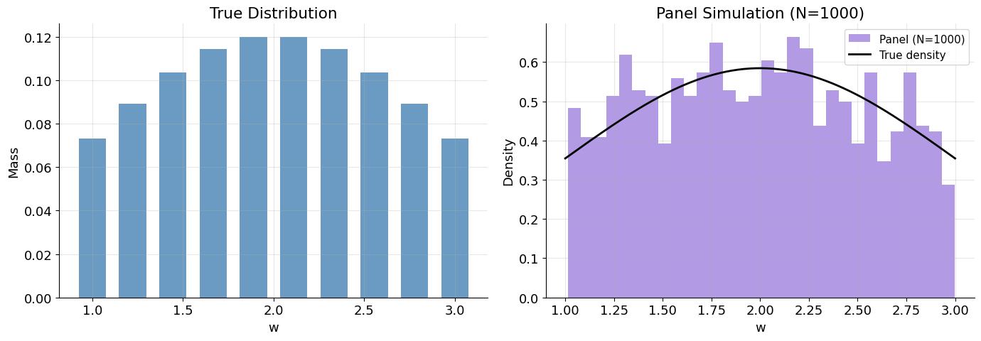
An alternative to Young’s histogram method is to simulate a panel of $N$ agents drawn from the distribution. The law of large numbers ensures that, for large $N$ , the sample moments converge to the true moments.

But how large does $N$ need to be?

# Draw a panel of agents from the truncated normal
np.random.seed(SEED + 42)
nb_agents = 1000
w_agents = dist.rvs(size=nb_agents)

# Compare moments
panel_mean = np.mean(w_agents)
panel_median = np.median(w_agents)
panel_var = np.var(w_agents)

print(f"Panel of {nb_agents} agents:")
print(f"{'':20s} {'True':>12s} {'Panel':>12s} {'Error':>12s}")
print("-" * 55)
print(f"{'Mean':20s} {true_mean:12.4f} {panel_mean:12.4f} {abs(true_mean-panel_mean):12.4f}")
print(f"{'Median':20s} {true_median:12.4f} {panel_median:12.4f} {abs(true_median-panel_median):12.4f}")
print(f"{'Variance':20s} {true_var:12.4f} {panel_var:12.4f} {abs(true_var-panel_var):12.4f}")

# Plot
fig, axes = plt.subplots(1, 2, figsize=(14, 5))

axes[0].bar(w_true, mass_true, width=0.15, alpha=0.8, color='steelblue', label='True distribution')
axes[0].set_xlabel('w')
axes[0].set_ylabel('Mass')
axes[0].set_title('True Distribution')

axes[1].hist(w_agents, bins=30, density=True, alpha=0.7, color='mediumpurple', label=f'Panel (N={nb_agents})')
# Overlay continuous true distribution
x_plot = np.linspace(w_true_lb, w_true_ub, 200)
axes[1].plot(x_plot, dist.pdf(x_plot), 'k-', linewidth=2, label='True density')
axes[1].set_xlabel('w')
axes[1].set_ylabel('Density')
axes[1].set_title(f'Panel Simulation (N={nb_agents})')
axes[1].legend(fontsize=11)

plt.tight_layout()
plt.show()

Panel of 1000 agents:
                             True        Panel        Error
-------------------------------------------------------
Mean                       2.0000       1.9818       0.0182
Median                     1.8889       1.9945       0.1056
Variance                   0.3465       0.2980       0.0485

7. Panel Convergence: How Many Agents Are Needed?¶

We increase the panel size from 1,000 to 100,000 and track how the sample mean converges to the true mean. The key insight: sampling error decays as $O(1/\sqrt{N})$ — you need a very large panel for accurate moments.

Young’s method, by contrast, has zero sampling error for the mean.

np.random.seed(SEED + 123)

# Panel sizes to try
panel_sizes = np.arange(1000, 100_001, 1000)
mean_panel = np.zeros(len(panel_sizes))
std_panel = np.zeros(len(panel_sizes))

# For each panel size, draw agents and compute sample mean
# We use a single large draw and take prefixes for consistency
all_agents = dist.rvs(size=100_000)

for i, n in enumerate(panel_sizes):
    sample = all_agents[:n]
    mean_panel[i] = np.mean(sample)
    std_panel[i] = np.std(sample) / np.sqrt(n)  # standard error of the mean

# 95% confidence interval
ci = 1.96 * std_panel

fig, ax = plt.subplots(figsize=(12, 6))
ax.fill_between(panel_sizes, mean_panel - ci, mean_panel + ci,
                alpha=0.3, color='steelblue', label='95% CI')
ax.plot(panel_sizes, mean_panel, '-', linewidth=1.5, color='steelblue', label='Panel mean')
ax.axhline(true_mean, color='crimson', linewidth=2, linestyle='--', label=f'True mean = {true_mean:.4f}')
ax.set_xlabel('Number of agents (N)')
ax.set_ylabel('Sample mean')
ax.set_title('Panel Simulation: Convergence of the Sample Mean')
ax.legend(fontsize=12)
plt.tight_layout()
plt.show()

print(f"Panel mean at N=1,000:   {mean_panel[0]:.6f}   (error = {abs(mean_panel[0]-true_mean):.6f})")
print(f"Panel mean at N=50,000:  {mean_panel[49]:.6f}   (error = {abs(mean_panel[49]-true_mean):.6f})")
print(f"Panel mean at N=100,000: {mean_panel[-1]:.6f}   (error = {abs(mean_panel[-1]-true_mean):.6f})")
print(f"\nYoung's method mean:     {approx_mean:.6f}   (error = {abs(approx_mean-true_mean):.2e})")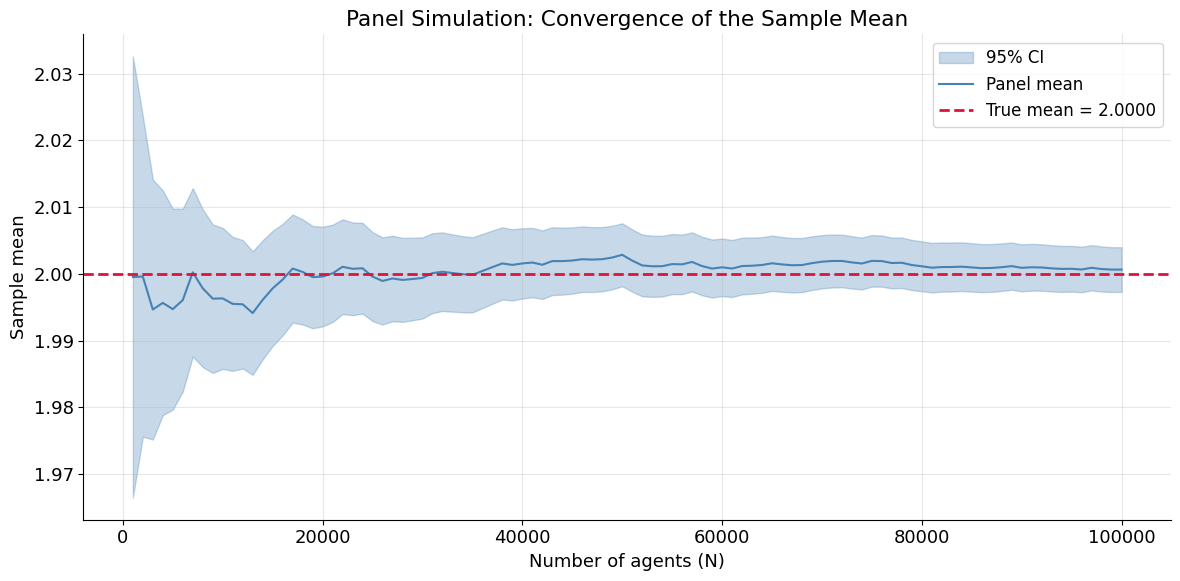

Panel mean at N=1,000:   1.999517   (error = 0.000483)
Panel mean at N=50,000:  2.002847   (error = 0.002847)
Panel mean at N=100,000: 2.000637   (error = 0.000637)

Young's method mean:     2.000000   (error = 0.00e+00)

8. Monte Carlo Comparison: Repeated Draws¶

To see the sampling noise more clearly, we repeat the panel simulation many times for different panel sizes and compare the standard deviation of the mean estimate.

np.random.seed(SEED + 456)

panel_sizes_mc = [500, 1000, 5000, 10_000, 50_000, 100_000]
n_replications = 200

results = {}
for n in panel_sizes_mc:
    means = np.array([np.mean(dist.rvs(size=n)) for _ in range(n_replications)])
    results[n] = means

fig, ax = plt.subplots(figsize=(12, 6))
positions = np.arange(len(panel_sizes_mc))
bp = ax.boxplot([results[n] for n in panel_sizes_mc], positions=positions,
                widths=0.5, patch_artist=True, showfliers=True)

colors = plt.cm.Blues(np.linspace(0.3, 0.8, len(panel_sizes_mc)))
for patch, color in zip(bp['boxes'], colors):
    patch.set_facecolor(color)

ax.axhline(true_mean, color='crimson', linewidth=2, linestyle='--', label=f'True mean = {true_mean:.4f}')
ax.set_xticks(positions)
ax.set_xticklabels([f'N={n:,}' for n in panel_sizes_mc], rotation=30)
ax.set_ylabel('Sample mean')
ax.set_title(f'Distribution of Panel Mean Across {n_replications} Replications')
ax.legend(fontsize=12, loc='upper right')
plt.tight_layout()
plt.show()

print(f"Standard deviation of mean estimate:")
for n in panel_sizes_mc:
    print(f"  N = {n:>7,}: std = {np.std(results[n]):.6f}")
print(f"\nYoung's method: std = 0 (deterministic)")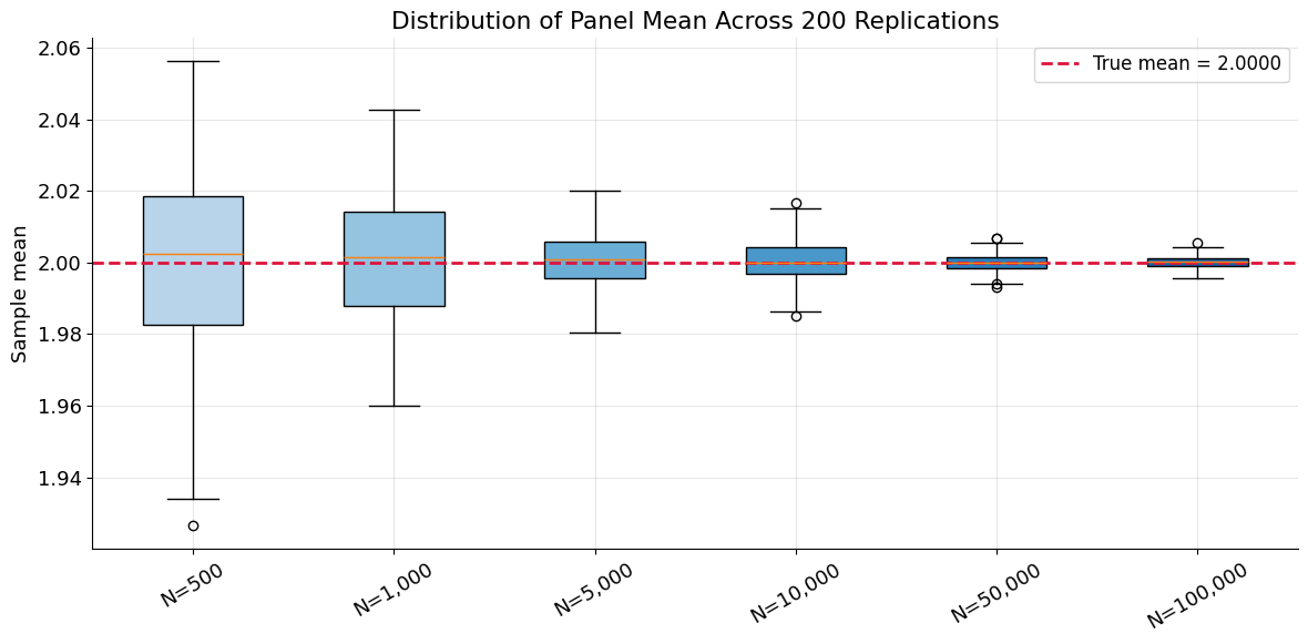

Standard deviation of mean estimate:
  N =     500: std = 0.024189
  N =   1,000: std = 0.016976
  N =   5,000: std = 0.008013
  N =  10,000: std = 0.005551
  N =  50,000: std = 0.002379
  N = 100,000: std = 0.001788

Young's method: std = 0 (deterministic)

9. Side-by-Side Comparison: Young vs. Panel¶

Let’s directly compare the two approaches for approximating the distribution.

np.random.seed(SEED + 789)

# Young's method with 20 grid points
n_young = 20
grid_young = np.linspace(0.5, 3.5, n_young)
hw_young = redistribute_distribution(w_true, mass_true, grid_young)

# Panel simulation with same number of "bins"
for n_panel in [100, 1_000, 10_000, 50_000]:
    w_panel = dist.rvs(size=n_panel)
    
    fig, axes = plt.subplots(1, 2, figsize=(14, 4.5))
    
    # Young's method
    axes[0].bar(grid_young, hw_young, width=0.12, alpha=0.8, color='steelblue',
                label=f"Young ({n_young} pts)")
    axes[0].bar(w_true, mass_true, width=0.06, alpha=0.5, color='orangered', label='True')
    axes[0].set_xlabel('w')
    axes[0].set_ylabel('Mass')
    axes[0].set_title(f"Young's Method ({n_young} grid points)")
    axes[0].legend(fontsize=10)
    axes[0].set_xlim(0.5, 3.5)
    
    # Panel histogram
    axes[1].hist(w_panel, bins=n_young, range=(0.5, 3.5), density=True, alpha=0.7,
                 color='mediumpurple', label=f'Panel (N={n_panel:,})')
    axes[1].plot(x_plot, dist.pdf(x_plot), 'k-', linewidth=2, label='True density')
    axes[1].set_xlabel('w')
    axes[1].set_ylabel('Density')
    axes[1].set_title(f'Panel Simulation (N={n_panel:,})')
    axes[1].legend(fontsize=10)
    axes[1].set_xlim(0.5, 3.5)
    
    # Annotate means
    young_mean = weighted_mean(grid_young, hw_young)
    panel_mean = np.mean(w_panel)
    axes[0].annotate(f'mean = {young_mean:.4f}', xy=(0.02, 0.95),
                     xycoords='axes fraction', fontsize=11, color='steelblue',
                     fontweight='bold', va='top')
    axes[1].annotate(f'mean = {panel_mean:.4f}', xy=(0.02, 0.95),
                     xycoords='axes fraction', fontsize=11, color='mediumpurple',
                     fontweight='bold', va='top')
    
    plt.suptitle(f'Young\'s Method vs. Panel Simulation', fontsize=13, y=1.02)
    plt.tight_layout()
    plt.show()
    
    print(f"N = {n_panel:>6,}:  Panel mean error = {abs(panel_mean - true_mean):.6f}, "
          f"Young mean error = {abs(young_mean - true_mean):.2e}")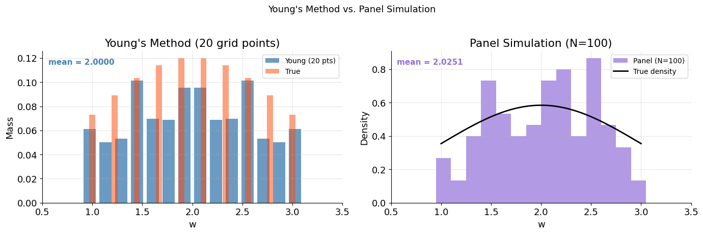

N =    100:  Panel mean error = 0.025053, Young mean error = 4.44e-16

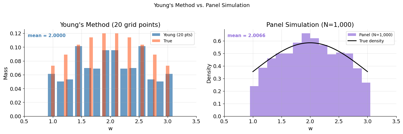
N =  1,000:  Panel mean error = 0.006575, Young mean error = 4.44e-16

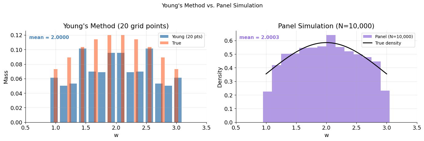
N = 10,000:  Panel mean error = 0.000303, Young mean error = 4.44e-16

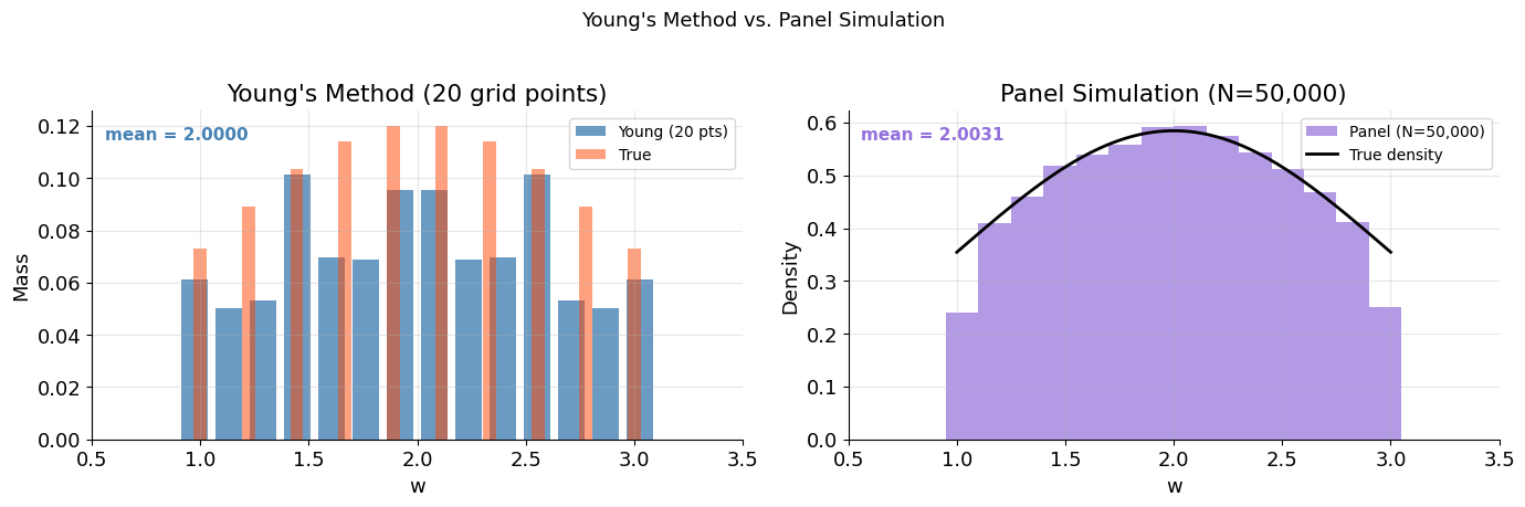
N = 50,000:  Panel mean error = 0.003061, Young mean error = 4.44e-16

10. Summary Comparison Table¶

print("\n" + "=" * 70)
print("           Young's Method vs. Panel Simulation")
print("=" * 70)
print(f"{'Property':<30s} {'Young (2010)':<20s} {'Panel (MC)':<20s}")
print("-" * 70)
print(f"{'Sampling noise':<30s} {'None':<20s} {'O(1/√N)':<20s}")
print(f"{'Mean preservation':<30s} {'Exact':<20s} {'Approximate':<20s}")
print(f"{'Higher moments':<30s} {'Approximate':<20s} {'Approximate':<20s}")
print(f"{'Deterministic':<30s} {'Yes':<20s} {'No':<20s}")
print(f"{'Resolution needed':<30s} {'~100-5000 grid pts':<20s} {'~50,000+ agents':<20s}")
print(f"{'Computational cost':<30s} {'Low':<20s} {'Higher':<20s}")
print(f"{'Differentiable':<30s} {'Yes (for DEQNs)':<20s} {'No':<20s}")
print("=" * 70)


======================================================================
           Young's Method vs. Panel Simulation
======================================================================
Property                       Young (2010)         Panel (MC)          
----------------------------------------------------------------------
Sampling noise                 None                 O(1/√N)             
Mean preservation              Exact                Approximate         
Higher moments                 Approximate          Approximate         
Deterministic                  Yes                  No                  
Resolution needed              ~100-5000 grid pts   ~50,000+ agents     
Computational cost             Low                  Higher              
Differentiable                 Yes (for DEQNs)      No                  
======================================================================

11. Dynamic Application: Forward Simulation with a Policy Function¶

In a heterogeneous agent model, we use Young’s method to propagate the distribution forward in time using the agents’ policy functions. Here we demonstrate with a simple savings policy.

Consider agents with wealth $k$ who save according to:

k' = g(k) = s \cdot k + (1 - s) \cdot \bar{k}

(3)

This is a linear policy that pushes wealth toward the mean $\bar{k}$ at rate $(1-s)$ .

def forward_step_young(grid, hist, policy_func):
    """
    One forward step of Young's method.
    
    Given a histogram on a grid and a policy function k' = g(k),
    compute the next-period histogram.
    """
    n = len(grid)
    new_hist = np.zeros(n)
    
    for i in range(n):
        if hist[i] < 1e-15:
            continue
        
        # Compute next-period value
        k_prime = policy_func(grid[i])
        
        # Find bracketing grid points
        j = np.searchsorted(grid, k_prime) - 1
        j = np.clip(j, 0, n - 2)
        
        # Boundary handling
        if k_prime <= grid[0]:
            new_hist[0] += hist[i]
        elif k_prime >= grid[-1]:
            new_hist[-1] += hist[i]
        else:
            # Interpolation weight
            w = 1.0 - (k_prime - grid[j]) / (grid[j + 1] - grid[j])
            w = np.clip(w, 0.0, 1.0)
            new_hist[j] += w * hist[i]
            new_hist[j + 1] += (1.0 - w) * hist[i]
    
    return new_hist


# Setup
n_grid_dyn = 50
k_grid = np.linspace(0.0, 10.0, n_grid_dyn)

# Initial distribution: uniform on [2, 8]
h0 = np.zeros(n_grid_dyn)
mask = (k_grid >= 2.0) & (k_grid <= 8.0)
h0[mask] = 1.0
h0 /= h0.sum()

# Policy: mean-reverting savings
s = 0.7  # persistence
k_bar = 5.0  # steady-state capital
policy = lambda k: s * k + (1 - s) * k_bar

# Simulate T periods
T = 30
hists = [h0]
means = [weighted_mean(k_grid, h0)]

for t in range(T):
    h_new = forward_step_young(k_grid, hists[-1], policy)
    hists.append(h_new)
    means.append(weighted_mean(k_grid, h_new))

# Plot distribution evolution
fig, axes = plt.subplots(2, 3, figsize=(15, 8))
plot_periods = [0, 1, 3, 5, 10, 29]
for ax, t_idx in zip(axes.flat, plot_periods):
    ax.bar(k_grid, hists[t_idx], width=0.15, color='steelblue', alpha=0.8)
    ax.axvline(means[t_idx], color='crimson', linewidth=2, linestyle='--')
    ax.set_title(f't = {t_idx}  (mean = {means[t_idx]:.3f})', fontsize=12)
    ax.set_xlim(-0.5, 10.5)
    ax.set_ylim(0, max(hists[t_idx]) * 1.3)
    ax.set_xlabel('k')

plt.suptitle("Young's Method: Distribution Evolution Under Mean-Reverting Policy",
             fontsize=14, y=1.02)
plt.tight_layout()
plt.show()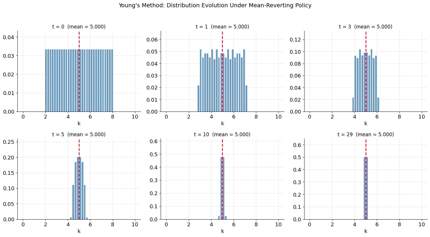

# Plot mean evolution
fig, ax = plt.subplots(figsize=(10, 5))
ax.plot(range(T + 1), means, 'o-', color='steelblue', linewidth=2, markersize=6)
ax.axhline(k_bar, color='crimson', linewidth=2, linestyle='--', label=f'Steady state $\\bar{{k}}$ = {k_bar}')
ax.set_xlabel('Period t')
ax.set_ylabel('Mean capital')
ax.set_title('Mean Capital Over Time (from Young\'s Forward Simulation)')
ax.legend(fontsize=12)
plt.tight_layout()
plt.show()

print(f"Mean at t=0:  {means[0]:.6f}")
print(f"Mean at t=30: {means[-1]:.6f}")
print(f"Steady state: {k_bar:.6f}")
print(f"\n→ Mean is preserved at {k_bar:.1f} throughout (as expected for this symmetric policy).")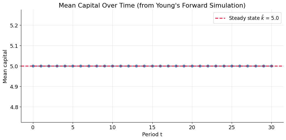

Mean at t=0:  5.000000
Mean at t=30: 5.000000
Steady state: 5.000000

→ Mean is preserved at 5.0 throughout (as expected for this symmetric policy).

12. With Idiosyncratic Shocks: Two Employment States¶

In a Krusell-Smith economy, agents face idiosyncratic employment shocks $\varepsilon \in \{e, u\}$ . The histogram is now 2D: mass at each $(k, \varepsilon)$ pair. Young’s method handles this by combining the policy-based mass redistribution with the Markov transition probabilities.

def forward_step_young_2d(grid, hist_2d, policy_funcs, trans_prob):
    """
    One forward step of Young's method with idiosyncratic shocks.
    
    Parameters
    ----------
    grid : array of shape (n_k,)
        Asset grid.
    hist_2d : array of shape (n_k, n_eps)
        Current histogram: hist_2d[i, j] = mass at (grid[i], eps_j).
    policy_funcs : list of callables
        policy_funcs[j](k) returns k' for employment state j.
    trans_prob : array of shape (n_eps, n_eps)
        Markov transition matrix: trans_prob[j, j'] = Prob(eps'=j' | eps=j).
    
    Returns
    -------
    new_hist : array of shape (n_k, n_eps)
    """
    n_k = len(grid)
    n_eps = hist_2d.shape[1]
    new_hist = np.zeros_like(hist_2d)
    
    for i in range(n_k):
        for eps in range(n_eps):
            if hist_2d[i, eps] < 1e-15:
                continue
            
            # Policy
            k_prime = policy_funcs[eps](grid[i])
            
            # Interpolation
            if k_prime <= grid[0]:
                j, w = 0, 1.0
            elif k_prime >= grid[-1]:
                j, w = n_k - 2, 0.0
            else:
                j = np.searchsorted(grid, k_prime) - 1
                j = np.clip(j, 0, n_k - 2)
                w = 1.0 - (k_prime - grid[j]) / (grid[j + 1] - grid[j])
                w = np.clip(w, 0.0, 1.0)
            
            # Redistribute across employment states
            for eps_next in range(n_eps):
                prob = trans_prob[eps, eps_next] * hist_2d[i, eps]
                new_hist[j, eps_next] += w * prob
                new_hist[j + 1, eps_next] += (1.0 - w) * prob
    
    return new_hist


# Setup
n_k = 100
k_grid = np.linspace(0.0, 20.0, n_k)

# Two employment states: employed (e) and unemployed (u)
# Transition matrix
pi_ee = 0.95  # prob staying employed
pi_uu = 0.90  # prob staying unemployed
trans_prob = np.array([
    [pi_ee, 1 - pi_ee],     # from employed
    [1 - pi_uu, pi_uu],     # from unemployed
])

# Policy functions (simple linear)
r = 0.04   # interest rate
w_e = 1.0  # wage when employed
w_u = 0.4  # wage when unemployed
delta = 0.05
s_rate = 0.3  # savings rate

policy_employed = lambda k: (1 + r - delta) * k * (1 - s_rate) + s_rate * ((1 + r - delta) * k + w_e)
# Simplify: k' = (1+r-delta)*k + w_e - c, where c = (1-s_rate)*((1+r-delta)*k + w_e)
# => k' = s_rate * ((1+r-delta)*k + w_e)
policy_e = lambda k: s_rate * ((1 + r - delta) * k + w_e)
policy_u = lambda k: s_rate * ((1 + r - delta) * k + w_u)

policy_funcs = [policy_e, policy_u]

# Initial distribution: everyone starts at k=5, half employed / half unemployed
hist_2d = np.zeros((n_k, 2))
idx_start = closest_index(k_grid, 5.0)
hist_2d[idx_start, 0] = 0.5  # employed
hist_2d[idx_start, 1] = 0.5  # unemployed

# Simulate
T = 100
hist_history = [hist_2d.copy()]
mean_k_history = [np.sum(k_grid[:, None] * hist_2d)]
frac_employed = [hist_2d[:, 0].sum()]

for t in range(T):
    hist_2d = forward_step_young_2d(k_grid, hist_2d, policy_funcs, trans_prob)
    hist_history.append(hist_2d.copy())
    mean_k_history.append(np.sum(k_grid[:, None] * hist_2d))
    frac_employed.append(hist_2d[:, 0].sum())

print(f"Stationary fraction employed: {frac_employed[-1]:.4f}")
print(f"  (Theoretical: {(1-pi_uu)/((1-pi_ee)+(1-pi_uu)):.4f})")
print(f"Mean capital at t={T}: {mean_k_history[-1]:.4f}")

Stationary fraction employed: 0.6667
  (Theoretical: 0.6667)
Mean capital at t=100: 0.3414

# Plot evolution of the 2D distribution
fig, axes = plt.subplots(2, 3, figsize=(16, 9))
plot_periods = [0, 5, 10, 20, 50, 100]

for ax, t_idx in zip(axes.flat, plot_periods):
    h = hist_history[t_idx]
    ax.bar(k_grid - 0.05, h[:, 0], width=0.1, alpha=0.8, color='steelblue', label='Employed')
    ax.bar(k_grid + 0.05, h[:, 1], width=0.1, alpha=0.8, color='orangered', label='Unemployed')
    ax.set_title(f't = {t_idx}', fontsize=12)
    ax.set_xlim(-0.5, 15)
    ax.set_xlabel('k')
    ax.set_ylabel('Mass')
    if t_idx == 0:
        ax.legend(fontsize=10)

plt.suptitle("Young's Method with Idiosyncratic Employment Shocks", fontsize=14, y=1.02)
plt.tight_layout()
plt.show()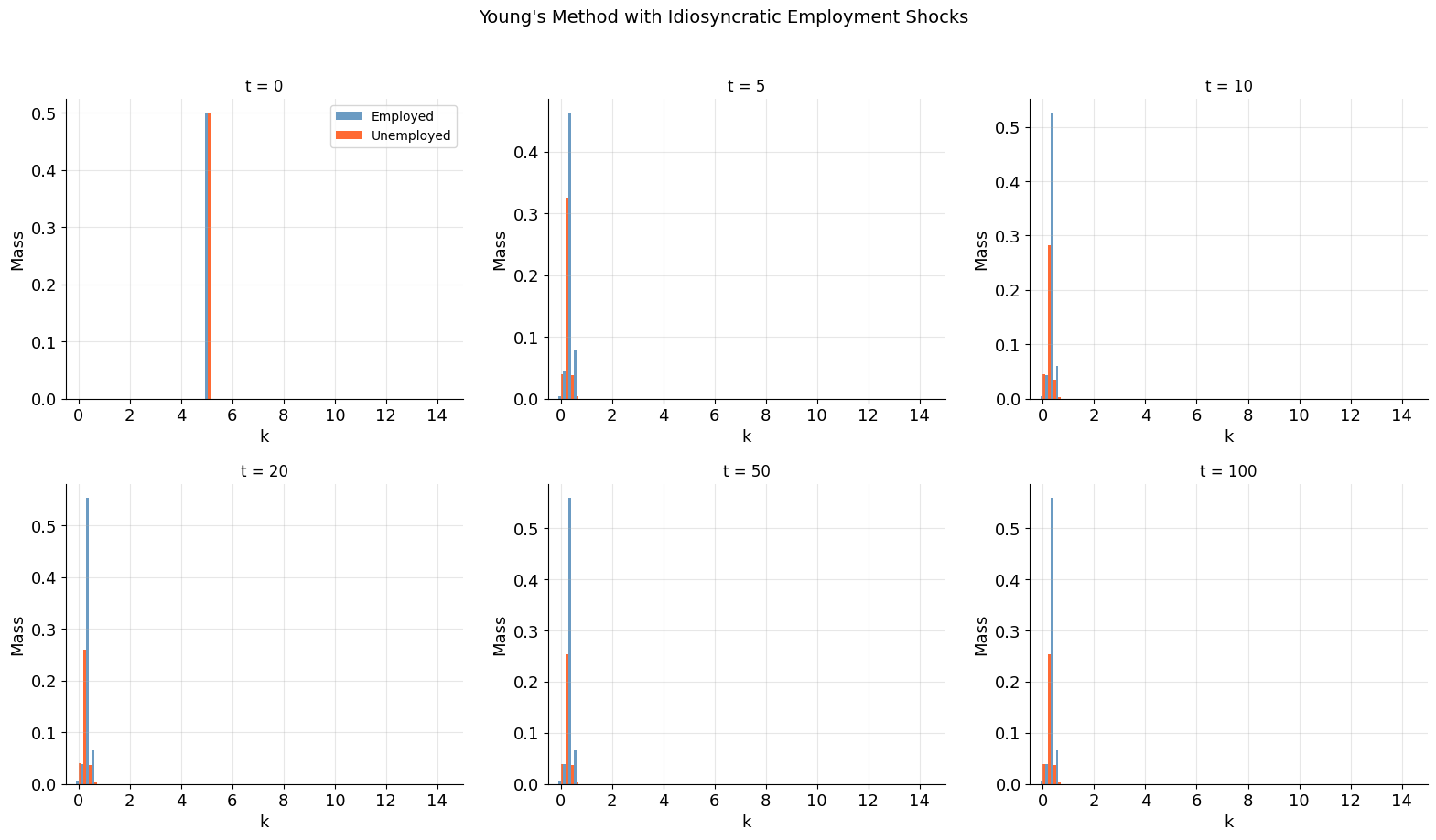

# Plot aggregate dynamics
fig, axes = plt.subplots(1, 2, figsize=(14, 5))

axes[0].plot(mean_k_history, 'o-', markersize=3, color='steelblue', linewidth=1.5)
axes[0].set_xlabel('Period')
axes[0].set_ylabel('Mean capital')
axes[0].set_title('Mean Capital Over Time')

axes[1].plot(frac_employed, 'o-', markersize=3, color='forestgreen', linewidth=1.5)
axes[1].axhline((1 - pi_uu) / ((1 - pi_ee) + (1 - pi_uu)), color='crimson',
               linestyle='--', linewidth=2, label='Stationary fraction')
axes[1].set_xlabel('Period')
axes[1].set_ylabel('Fraction employed')
axes[1].set_title('Employment Rate Over Time')
axes[1].legend(fontsize=12)

plt.suptitle('Aggregate Dynamics from Young\'s Forward Simulation', fontsize=14, y=1.02)
plt.tight_layout()
plt.show()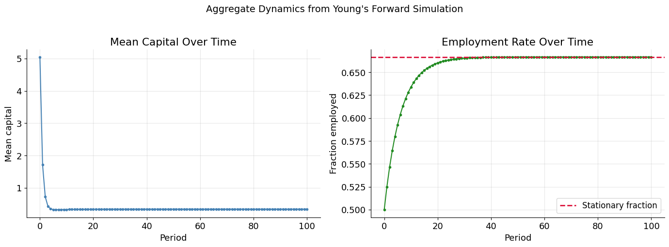

# Final stationary-ish distribution
h_final = hist_history[-1]

fig, ax = plt.subplots(figsize=(12, 6))
ax.bar(k_grid - 0.05, h_final[:, 0], width=0.1, alpha=0.8, color='steelblue', label='Employed')
ax.bar(k_grid + 0.05, h_final[:, 1], width=0.1, alpha=0.8, color='orangered', label='Unemployed')
ax.axvline(mean_k_history[-1], color='black', linewidth=2, linestyle='--',
           label=f'Mean = {mean_k_history[-1]:.2f}')
ax.set_xlabel('Capital k', fontsize=13)
ax.set_ylabel('Mass', fontsize=13)
ax.set_title(f'Stationary Distribution (t = {T})', fontsize=14)
ax.set_xlim(-0.5, 12)
ax.legend(fontsize=12)
plt.tight_layout()
plt.show()

# Distributional statistics
total_mass_e = h_final[:, 0].sum()
total_mass_u = h_final[:, 1].sum()
mean_k_e = np.average(k_grid, weights=h_final[:, 0]) if total_mass_e > 0 else 0
mean_k_u = np.average(k_grid, weights=h_final[:, 1]) if total_mass_u > 0 else 0

print(f"\nStationary Distribution Statistics:")
print(f"  Overall mean capital:     {mean_k_history[-1]:.4f}")
print(f"  Mean capital (employed):  {mean_k_e:.4f}")
print(f"  Mean capital (unemployed):{mean_k_u:.4f}")
print(f"  Fraction employed:        {total_mass_e:.4f}")
print(f"  Fraction unemployed:      {total_mass_u:.4f}")
print(f"  Total mass:               {h_final.sum():.6f}  (should be 1.0)")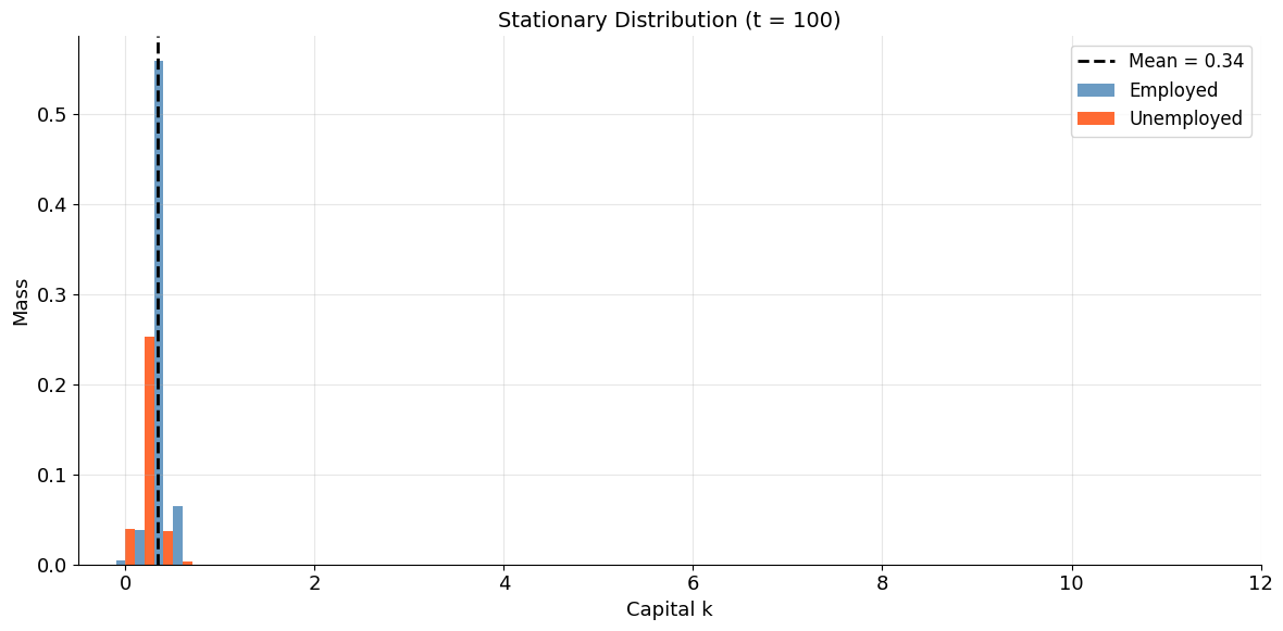


Stationary Distribution Statistics:
  Overall mean capital:     0.3414
  Mean capital (employed):  0.4096
  Mean capital (unemployed):0.2049
  Fraction employed:        0.6667
  Fraction unemployed:      0.3333
  Total mass:               1.000000  (should be 1.0)

12b. Reproducing the Script’s Worked 4-Point Example¶

Chapter 6, §6.3 walks through a hand-worked Young update on a tiny grid. We reproduce it here with forward_step_young_2d and check the printed histograms and means against the script.

Setup. Grid $\{1,2,3,4\}$ , two idiosyncratic states $\{\text{low},\text{high}\}$ , savings rule $k' = 0.4\,k + 0.5\,y(\varepsilon)$ with $y_\text{low}=1$ , $y_\text{high}=3$ , and an identity shock transition. The initial histogram $G_0$ has masses $(0.10,0.20,0.10,0.05)$ in the low row and $(0.05,0.15,0.20,0.15)$ in the high row, so $\bar k_0 = 2.55$ . The script reports $\bar k_1 = 2.08$ , with the unclipped policy-implied mean equal to 2.07 (boundary clipping at $k'=0.9$ adds $\approx 0.01$ ).

# Script's 4-point worked example (Chapter 6, Young's non-stochastic simulation)
g4 = np.array([1.0, 2.0, 3.0, 4.0])

# Initial histogram G0[k_idx, eps_idx]; column 0 = low, column 1 = high
G0 = np.array([
    [0.10, 0.05],   # k = 1
    [0.20, 0.15],   # k = 2
    [0.10, 0.20],   # k = 3
    [0.05, 0.15],   # k = 4
])
assert np.isclose(G0.sum(), 1.0)

# Savings rule k' = 0.4 k + 0.5 y(eps);  y_low = 1, y_high = 3
y4 = [1.0, 3.0]
pol4 = [lambda k: 0.4 * k + 0.5 * y4[0],   # low state
        lambda k: 0.4 * k + 0.5 * y4[1]]   # high state

# Identity shock transition (matches the script's Step 4)
I2 = np.eye(2)

G1 = forward_step_young_2d(g4, G0, pol4, I2)

kbar0 = float(np.sum(g4[:, None] * G0))
kbar1 = float(np.sum(g4[:, None] * G1))
kprime_implied = sum(G0[i, e] * pol4[e](g4[i]) for i in range(4) for e in range(2))

print('G1  (rows = k in {1,2,3,4}, cols = [low, high]):')
print(np.round(G1, 3))
print(f'\nrow sums:  low = {G1[:, 0].sum():.3f},  high = {G1[:, 1].sum():.3f},  total = {G1.sum():.3f}')
print(f'\nmean capital  k_bar_0 = {kbar0:.2f}   (script: 2.55)')
print(f'mean capital  k_bar_1 = {kbar1:.2f}   (script: 2.08)')
print(f'unclipped policy-implied mean = {kprime_implied:.2f}   (script: 2.07)')
print('-> boundary clipping at k\' = 0.9 raises the next-period mean by ~0.01, exactly as the script notes.')

G1  (rows = k in {1,2,3,4}, cols = [low, high]):
[[0.27  0.005]
 [0.175 0.21 ]
 [0.005 0.32 ]
 [0.    0.015]]

row sums:  low = 0.450,  high = 0.550,  total = 1.000

mean capital  k_bar_0 = 2.55   (script: 2.55)
mean capital  k_bar_1 = 2.08   (script: 2.08)
unclipped policy-implied mean = 2.07   (script: 2.07)
-> boundary clipping at k' = 0.9 raises the next-period mean by ~0.01, exactly as the script notes.

13. The Cascading Fork: One Cell Splits into Four¶

The 2D Young step in section 12 already combines the capital lottery (split off-grid $k'$ between $k_J$ and $k_{J+1}$ ) with the shock fork (transition from $\varepsilon$ to $\varepsilon'$ via $\pi_{\varepsilon\varepsilon'}$ ). This section makes the two-stage cascade explicit on a single source bin, matching the four-leaf cascade figure (fig:young_cascade) in §6.3 of the script (essentially Fig. 1 of Young 2010) and the corresponding “one cell splits into four” slide of the L10 deck.

Setup (matches the script’s worked example). One source mass $m=0.05$ at $(k, \varepsilon=L)$ . Capital lottery weights $\omega=0.6$ , $1-\omega=0.4$ . Shock fork $\pi_{LL}=0.9$ , $\pi_{LH}=0.1$ .

Expected leaves (product of stage-1 and stage-2 weights):

$(k_J, L)$ : $0.6 \times 0.9 \times 0.05 = 0.027$
$(k_J, H)$ : $0.6 \times 0.1 \times 0.05 = 0.003$
$(k_{J+1}, L)$ : $0.4 \times 0.9 \times 0.05 = 0.018$
$(k_{J+1}, H)$ : $0.4 \times 0.1 \times 0.05 = 0.002$

Sum: $0.027 + 0.003 + 0.018 + 0.002 = 0.05 = m$ . Mass conservation by construction.

# Cascading fork: one source cell -> four destination leaves.
# Stage 1 (capital lottery): split mass between bracketing grid points.
# Stage 2 (shock fork): split each piece across reachable next-period eps'.

m_source = 0.05            # mass at the source bin
omega = 0.6                # capital-lottery weight on the lower bracket k_J
pi = np.array([[0.9, 0.1], # pi[L, L'], pi[L, H'] -- the source eps is L
               [0.2, 0.8]])

# Source state index: eps_src = 0 (low)
eps_src = 0

# The four leaf masses, by hand:
leaves = {
    '(k_J,    L)': omega       * pi[eps_src, 0] * m_source,
    '(k_J,    H)': omega       * pi[eps_src, 1] * m_source,
    '(k_J+1,  L)': (1 - omega) * pi[eps_src, 0] * m_source,
    '(k_J+1,  H)': (1 - omega) * pi[eps_src, 1] * m_source,
}

for label, mass in leaves.items():
    print(f'  {label:<14s} = {mass:.4f}')

total = sum(leaves.values())
print(f'\n  sum of leaves = {total:.4f}   (source mass m = {m_source:.4f})')

# Stage-1 mean preservation: omega * k_J + (1 - omega) * k_{J+1} = k'.
# Demonstrate with a concrete grid:
k_J, k_Jp1 = 2.0, 4.0
k_prime    = omega * k_J + (1 - omega) * k_Jp1
print(f'\n  stage-1 conditional mean: omega*k_J + (1-omega)*k_(J+1) = {k_prime:.3f}')
print('  (matches the off-grid policy choice k_prime by construction)')

  (k_J,    L)    = 0.0270
  (k_J,    H)    = 0.0030
  (k_J+1,  L)    = 0.0180
  (k_J+1,  H)    = 0.0020

  sum of leaves = 0.0500   (source mass m = 0.0500)

  stage-1 conditional mean: omega*k_J + (1-omega)*k_(J+1) = 2.800
  (matches the off-grid policy choice k_prime by construction)

Conclusion¶

This notebook demonstrated Young’s (2010) non-stochastic simulation method:

Core algorithm: Linear interpolation to redistribute mass on a fixed grid
Mean preservation: The method preserves the mean of the distribution exactly
Higher moments: Variance and median are approximated; finer grids → better accuracy
No sampling noise: Unlike panel simulation, which requires tens of thousands of agents
Forward simulation: Can propagate distributions forward in time using policy functions
Idiosyncratic shocks: Naturally extends to multiple employment/income states

Bridge to `11_Continuum_of_Agents_DEQN`¶

The toy object h(k) becomes a stacked histogram over $(\eta, b)$ blocks
The hand-set policy function becomes a policy network output $b'(\eta, b, x_t^{agg})$
The weighted mean calculation becomes exact market clearing via the histogram dot product with network-implied savings

Next steps¶

Combine with value function iteration (or neural networks) to solve full heterogeneous agent models
Use as the distribution propagation step inside DEQN training loops
See the companion slides: lecture_09_heterogeneous_agents_youngs.pdf

Reference¶

Young, E.R. (2010). “Solving the incomplete markets model with aggregate uncertainty using the Krusell–Smith algorithm and non-stochastic simulations.” Journal of Economic Dynamics and Control, 34(1), 36–41.