Course: Deep Learning for Solving and Estimating Dynamic Models in Economics and Finance
Script reference: §3.2 (model setup), §3.3 (Euler equation and aggregate resource constraint), §3.4 (smooth DEQN loss, network architecture), §3.5 (persistent-simulation training; time-invariance and zero-shock stochastic-steady-state diagnostics)
Notebook role: core
Author: Simon Scheidegger
RUN_MODE = "smoke"  # one of: "smoke", "teaching", "production"
SEED = 0
This notebook solves the smooth -country international real business-cycle model with complete markets, productivity risk, and convex capital-adjustment costs. It is deliberately written as a teaching notebook: one model, one training loop, and one switch between simulation-based and exogenous training states.
The central design choice is in the construction of the training data. In simulation mode the notebook does not restart from the steady state in every episode. Instead, it keeps a vector of current trajectory heads. Each training segment simulates these trajectory heads forward for SIMULATION_LENGTH stochastic periods, flattens the simulated states into a training cloud, performs the chosen stochastic-gradient updates, and then continues from the terminal states of the same trajectories.
The state is
The policy network returns only
because this smooth benchmark has no irreversible-investment multipliers.
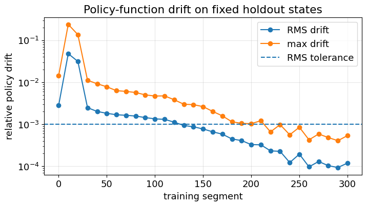
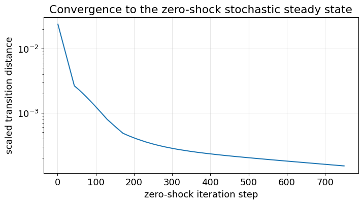
Two additional diagnostics are included. The first monitors whether the learned policy has stabilized across training iterations by measuring policy drift on a fixed holdout cloud. The second computes the zero-shock stochastic steady state: the fixed point of the learned stochastic policy when realized shocks are set to zero.
# ============================================================
# Imports, run-mode switch, and configuration (RUN_MODE/SEED from cell 2)
# ============================================================
import math
import numpy as np
import tensorflow as tf
from tensorflow import keras
import matplotlib.pyplot as plt

plt.rcParams["font.size"] = 13

np.random.seed(SEED)
tf.random.set_seed(SEED)
rng = np.random.default_rng(SEED)

# ------------------------------------------------------------
# Training-data switch
# ------------------------------------------------------------
# "simulation": simulate trajectories under the current policy and train on
#               the states visited by those trajectories.
# "exogenous" : ignore the simulated trajectory heads and draw states from
#               a user-chosen rectangular box.
SAMPLING_MODE = "simulation"       # "simulation" or "exogenous"

# ------------------------------------------------------------
# Training-budget switch
# ------------------------------------------------------------
# The examples below illustrate the intended use.
#   One long trajectory:        N_TRAJECTORIES = 1,  SIMULATION_LENGTH = 1024
#   Several shorter tracks:     N_TRAJECTORIES = 10, SIMULATION_LENGTH = 256
# In both cases each trajectory receives its own idiosyncratic shocks.

if RUN_MODE == "smoke":
    NUM_SEGMENTS = 25
    N_TRAJECTORIES = 4
    SIMULATION_LENGTH = 32
    BATCH_SIZE = 128
    LEARNING_RATE = 3e-4
    MONITOR_EVERY = 5
elif RUN_MODE == "teaching":
    NUM_SEGMENTS = 301
    N_TRAJECTORIES = 10
    SIMULATION_LENGTH = 256
    BATCH_SIZE = 512
    LEARNING_RATE = 2e-4
    MONITOR_EVERY = 10
elif RUN_MODE == "production":
    NUM_SEGMENTS = 1201
    N_TRAJECTORIES = 32
    SIMULATION_LENGTH = 512
    BATCH_SIZE = 1024
    LEARNING_RATE = 1e-4
    MONITOR_EVERY = 25
else:
    raise ValueError(f"Unknown RUN_MODE: {RUN_MODE}")

# How many passes over one simulated segment before we move to the next
# segment.  The baseline DEQN style is PASSES_PER_SEGMENT = 1.
PASSES_PER_SEGMENT = 1
SHUFFLE_STATES_WITHIN_SEGMENT = True

# Optimizer choices.  Supported names: "Adam", "AdamW", "RMSprop", "SGD".
OPTIMIZER_NAME = "Adam"
ADAM_BETA_1 = 0.9
ADAM_BETA_2 = 0.999
RMSPROP_RHO = 0.9
SGD_MOMENTUM = 0.0
WEIGHT_DECAY = 0.0               # used only by AdamW if selected
CLIP_NORM = 10.0                 # set to None to disable global gradient clipping

# Loss weights.  The residuals are already dimensionless, so unit weights
# are meaningful starting values.
EULER_WEIGHT = 1.0
ARC_WEIGHT = 1.0

# Exogenous training draws use the same number of states as one simulated
# segment, so switching SAMPLING_MODE does not change the batch scale.
EXOGENOUS_STATES_PER_SEGMENT = N_TRAJECTORIES * SIMULATION_LENGTH

# Emergency repair is not a scheduled reset.  It only replaces a trajectory
# if numerical training produces a non-finite or wildly out-of-domain state.
# The replacement state is drawn from the feasible initial-state box below,
# not from the steady state.
EMERGENCY_REPAIR_BAD_STATES = True
SIM_REPAIR_K_MIN = 0.05
SIM_REPAIR_K_MAX = 8.0
SIM_REPAIR_ABS_Z_MAX_MULTIPLE = 8.0

# ------------------------------------------------------------
# Convergence diagnostics: policy drift and zero-shock steady state
# ------------------------------------------------------------
# A feed-forward policy network without calendar time as an input is
# time-homogeneous by construction.  The economically relevant check is
# whether the *learned function* has stopped changing across SGD updates.
# We therefore evaluate policies on a fixed anchor cloud that is never used
# for training and monitor the monitor-to-monitor policy drift.
if RUN_MODE == "smoke":
    TIME_INVARIANCE_ANCHOR_STATES = 256
    ZERO_SHOCK_N_STARTS = 8
    ZERO_SHOCK_MAX_STEPS = 250
elif RUN_MODE == "teaching":
    TIME_INVARIANCE_ANCHOR_STATES = 2048
    ZERO_SHOCK_N_STARTS = 32
    ZERO_SHOCK_MAX_STEPS = 750
elif RUN_MODE == "production":
    TIME_INVARIANCE_ANCHOR_STATES = 4096
    ZERO_SHOCK_N_STARTS = 64
    ZERO_SHOCK_MAX_STEPS = 1500
else:
    raise ValueError(f"Unknown RUN_MODE: {RUN_MODE}")

TIME_INVARIANCE_TOL_RMS = 1.0e-3
TIME_INVARIANCE_TOL_MAX = 1.0e-2

# The stochastic steady state is computed as the fixed point of the learned
# stochastic policy when the realized shocks are set to zero.  This is not
# the deterministic steady state of the non-stochastic economy; the policy
# still embodies the stochastic Euler equations.
RUN_ZERO_SHOCK_STEADY_STATE_CHECK = True
ZERO_SHOCK_TOL = 1.0e-7
ZERO_SHOCK_FIXED_POINT_TOL = 1.0e-4
ZERO_SHOCK_Z_TOL = 1.0e-4
ZERO_SHOCK_CROSS_TRACK_TOL = 5.0e-3
SSS_MEAN_RESIDUAL_TOL = 1.0e-2
SSS_K_MIN_OK = 0.20
SSS_K_MAX_OK = 5.00

print(f"TensorFlow version: {tf.__version__}")
print(f"SAMPLING_MODE = {SAMPLING_MODE}")
print(f"RUN_MODE = {RUN_MODE}")
print(f"N_TRAJECTORIES = {N_TRAJECTORIES}")
print(f"SIMULATION_LENGTH = {SIMULATION_LENGTH}")
print(f"states per segment = {N_TRAJECTORIES * SIMULATION_LENGTH}")
print(f"optimizer = {OPTIMIZER_NAME}, learning rate = {LEARNING_RATE}")
print(f"batch size = {BATCH_SIZE}, passes per segment = {PASSES_PER_SEGMENT}")
print(f"time-invariance anchor states = {TIME_INVARIANCE_ANCHOR_STATES}")
print(f"zero-shock starts = {ZERO_SHOCK_N_STARTS}, max steps = {ZERO_SHOCK_MAX_STEPS}")
2026-05-05 21:48:06.352422: I tensorflow/core/util/port.cc:153] oneDNN custom operations are on. You may see slightly different numerical results due to floating-point round-off errors from different computation orders. To turn them off, set the environment variable `TF_ENABLE_ONEDNN_OPTS=0`.
2026-05-05 21:48:06.367599: I external/local_xla/xla/tsl/cuda/cudart_stub.cc:32] Could not find cuda drivers on your machine, GPU will not be used.
2026-05-05 21:48:06.459948: I external/local_xla/xla/tsl/cuda/cudart_stub.cc:32] Could not find cuda drivers on your machine, GPU will not be used.
2026-05-05 21:48:06.529222: E external/local_xla/xla/stream_executor/cuda/cuda_fft.cc:467] Unable to register cuFFT factory: Attempting to register factory for plugin cuFFT when one has already been registered
WARNING: All log messages before absl::InitializeLog() is called are written to STDERR
E0000 00:00:1778010486.602085    8726 cuda_dnn.cc:8579] Unable to register cuDNN factory: Attempting to register factory for plugin cuDNN when one has already been registered
E0000 00:00:1778010486.625014    8726 cuda_blas.cc:1407] Unable to register cuBLAS factory: Attempting to register factory for plugin cuBLAS when one has already been registered
W0000 00:00:1778010486.781268    8726 computation_placer.cc:177] computation placer already registered. Please check linkage and avoid linking the same target more than once.
W0000 00:00:1778010486.781310    8726 computation_placer.cc:177] computation placer already registered. Please check linkage and avoid linking the same target more than once.
W0000 00:00:1778010486.781312    8726 computation_placer.cc:177] computation placer already registered. Please check linkage and avoid linking the same target more than once.
W0000 00:00:1778010486.781314    8726 computation_placer.cc:177] computation placer already registered. Please check linkage and avoid linking the same target more than once.
2026-05-05 21:48:06.800809: I tensorflow/core/platform/cpu_feature_guard.cc:210] This TensorFlow binary is optimized to use available CPU instructions in performance-critical operations.
To enable the following instructions: AVX2 AVX_VNNI FMA, in other operations, rebuild TensorFlow with the appropriate compiler flags.
TensorFlow version: 2.19.0
SAMPLING_MODE = simulation
MODE = teaching
N_TRAJECTORIES = 10
SIMULATION_LENGTH = 256
states per segment = 2560
optimizer = Adam, learning rate = 0.0002
batch size = 512, passes per segment = 1
time-invariance anchor states = 2048
zero-shock starts = 32, max steps = 750
1. Economic parameters¶
Productivity is represented by and follows
The innovation variance of is therefore , which is used below to create reasonable productivity boxes for exogenous sampling and for the initial trajectory heads.
The deterministic normalization sets the reference capital level to one. The simulated training data below does not start from that reference point; the reference level is used only to scale neural-network inputs and complete-markets weights.
# ============================================================
# IRBC parameters
# ============================================================
N_COUNTRIES = 2

beta = 0.99
zeta = 0.36
delta = 0.01
rho_z = 0.95
sigma_e = 0.01
kappa = 0.50

gamma_min = 0.25
gamma_max = 1.00

# Reference capital level.  In the Brumm--Scheidegger / Den Haan et al.
# normalization, A is chosen so that the deterministic steady-state capital
# is one.  We do not use this as a repeated simulation start.
K_REF = 1.0
LAMBDA_REF = 1.0

# Deterministic Euler equation at k=K_REF, z=0, and k'=k:
#   1 = beta * (A*zeta*K_REF^(zeta-1) + 1 - delta).
A_tfp = (1.0 / beta - 1.0 + delta) / (zeta * K_REF ** (zeta - 1.0))
Y_ref = A_tfp * K_REF ** zeta
C_ref = Y_ref - delta * K_REF

if N_COUNTRIES == 1:
    gammas_np = np.array([gamma_min], dtype=np.float32)
else:
    gammas_np = np.linspace(gamma_min, gamma_max, N_COUNTRIES, dtype=np.float32)

# Complete-markets FOC: tau_j * c_j^(-1/gamma_j) = lambda.
# The following choice gives c_j=C_ref when lambda=LAMBDA_REF.
taus_np = LAMBDA_REF * C_ref ** (1.0 / gammas_np)

gammas_tf = tf.constant(gammas_np.reshape(1, N_COUNTRIES), dtype=tf.float32)
taus_tf = tf.constant(taus_np.reshape(1, N_COUNTRIES), dtype=tf.float32)

n_states = 2 * N_COUNTRIES      # [k_1,...,k_N,z_1,...,z_N]
n_policies = N_COUNTRIES + 1    # [k'_1,...,k'_N,lambda]
n_shocks = N_COUNTRIES + 1      # N idiosyncratic shocks + one aggregate shock

z_std = sigma_e * math.sqrt(2.0 / (1.0 - rho_z ** 2))
z_bound = 3.0 * z_std

# Exogenous sampling box.
EXOGENOUS_K_LOW = 0.55
EXOGENOUS_K_HIGH = 1.80
EXOGENOUS_Z_LOW = -z_bound
EXOGENOUS_Z_HIGH = z_bound

# Initial trajectory heads for simulation-based training.
# These are deliberately feasible and dispersed.  They are not steady-state starts.
INITIAL_K_LOW = 0.65
INITIAL_K_HIGH = 1.45
INITIAL_Z_LOW = -1.5 * z_std
INITIAL_Z_HIGH = 1.5 * z_std

SIM_REPAIR_ABS_Z_MAX = SIM_REPAIR_ABS_Z_MAX_MULTIPLE * z_std

print("=== Smooth IRBC parameters ===")
print(f"N_COUNTRIES = {N_COUNTRIES}")
print(f"states = {n_states}, policies = {n_policies}, shocks = {n_shocks}")
print(f"A_tfp = {A_tfp:.6f}, Y_ref = {Y_ref:.6f}, C_ref = {C_ref:.6f}")
print(f"gammas = {gammas_np}")
print(f"taus = {taus_np}")
print(f"z_std = {z_std:.5f}")
print(f"exogenous k box = [{EXOGENOUS_K_LOW}, {EXOGENOUS_K_HIGH}]")
print(f"exogenous z box = [{EXOGENOUS_Z_LOW:.5f}, {EXOGENOUS_Z_HIGH:.5f}]")
print(f"initial k box = [{INITIAL_K_LOW}, {INITIAL_K_HIGH}]")
print(f"initial z box = [{INITIAL_Z_LOW:.5f}, {INITIAL_Z_HIGH:.5f}]")
=== Smooth IRBC parameters ===
N_COUNTRIES = 2
states = 4, policies = 3, shocks = 3
A_tfp = 0.055836, Y_ref = 0.055836, C_ref = 0.045836
gammas = [0.25 1.  ]
taus = [4.413998e-06 4.583614e-02]
z_std = 0.04529
exogenous k box = [0.55, 1.8]
exogenous z box = [-0.13587, 0.13587]
initial k box = [0.65, 1.45]
initial z box = [-0.06794, 0.06794]
E0000 00:00:1778010493.510424    8726 cuda_executor.cc:1228] INTERNAL: CUDA Runtime error: Failed call to cudaGetRuntimeVersion: Error loading CUDA libraries. GPU will not be used.: Error loading CUDA libraries. GPU will not be used.
W0000 00:00:1778010493.513171    8726 gpu_device.cc:2341] Cannot dlopen some GPU libraries. Please make sure the missing libraries mentioned above are installed properly if you would like to use GPU. Follow the guide at https://www.tensorflow.org/install/gpu for how to download and setup the required libraries for your platform.
Skipping registering GPU devices...
2. Integration rule¶
The expectation in the Euler equations is evaluated with a monomial rule. It uses nodes instead of a tensor-product Gauss--Hermite rule with nodes, so it remains cheap when the number of countries increases.
def make_monomial_rule(dim):
    """Monomial rule for E[f(eps)] with eps ~ N(0,I_dim).

    The nodes are +/-sqrt(dim) along each coordinate axis, each with weight
    1/(2*dim).  The rule exactly integrates constants, first moments, and
    second moments of a standard normal vector.
    """
    radius = math.sqrt(dim)
    nodes = []
    weights = []
    for i in range(dim):
        e = np.zeros(dim, dtype=np.float32)
        e[i] = radius
        nodes.append(e.copy())
        e[i] = -radius
        nodes.append(e.copy())
        weights.extend([1.0 / (2.0 * dim), 1.0 / (2.0 * dim)])
    return np.asarray(nodes, dtype=np.float32), np.asarray(weights, dtype=np.float32)

quad_nodes_np, quad_weights_np = make_monomial_rule(n_shocks)
quad_nodes_tf = tf.constant(quad_nodes_np, dtype=tf.float32)
quad_weights_tf = tf.constant(quad_weights_np.reshape(-1, 1), dtype=tf.float32)
n_quad = quad_nodes_np.shape[0]

print(f"quadrature nodes = {n_quad}")
print(f"sum of quadrature weights = {quad_weights_np.sum():.6f}")
quadrature nodes = 6
sum of quadrature weights = 1.000000
3. Neural network and policy transformation¶
The network is initialized so that and before training. This is not a training-data assumption; it is only a stable initial policy. Next-period capital is parameterized relative to current capital:
Thus remains positive and per-period capital growth is bounded during simulation.
# Input and output scales.
INPUT_K_LOG_SCALE = 0.50
INPUT_Z_SCALE = max(z_bound, 1e-6)
KP_GROWTH_SCALE = 0.30       # |log(k'/k)| <= 0.30 per simulated step
LAMBDA_LOG_SCALE = 1.25

NUM_HIDDEN_1 = 128
NUM_HIDDEN_2 = 128
ACTIVATION = "tanh"

def scale_states(states):
    """Scale states before passing them to the neural network."""
    states = tf.convert_to_tensor(states, dtype=tf.float32)
    k = tf.maximum(states[:, :N_COUNTRIES], 1e-8)
    z = states[:, N_COUNTRIES:]
    k_scaled = tf.math.log(k / K_REF) / INPUT_K_LOG_SCALE
    z_scaled = z / INPUT_Z_SCALE
    return tf.concat([k_scaled, z_scaled], axis=1)

def build_network():
    """Build a policy network with zero last layer.

    With the policy transformation below, zero raw outputs imply k'=k and
    lambda=1.  This makes early simulation stable even when initial states
    are dispersed.
    """
    return keras.Sequential([
        keras.layers.Input(shape=(n_states,)),
        keras.layers.Dense(NUM_HIDDEN_1, activation=ACTIVATION),
        keras.layers.Dense(NUM_HIDDEN_2, activation=ACTIVATION),
        keras.layers.Dense(
            n_policies,
            activation=None,
            kernel_initializer="zeros",
            bias_initializer="zeros",
        ),
    ])

def policy(states, model):
    """Map states to economically admissible smooth-model policies."""
    states = tf.convert_to_tensor(states, dtype=tf.float32)
    k = tf.maximum(states[:, :N_COUNTRIES], 1e-8)
    raw = model(scale_states(states))
    raw_k = raw[:, :N_COUNTRIES]
    raw_lambda = raw[:, N_COUNTRIES:N_COUNTRIES + 1]

    kp = k * tf.exp(KP_GROWTH_SCALE * tf.tanh(raw_k))
    lamb = LAMBDA_REF * tf.exp(LAMBDA_LOG_SCALE * tf.tanh(raw_lambda))
    return kp, lamb

model_check = build_network()
X_check = tf.constant(np.concatenate([
    np.ones((3, N_COUNTRIES), dtype=np.float32),
    np.zeros((3, N_COUNTRIES), dtype=np.float32),
], axis=1))
kp_check, lambda_check = policy(X_check, model_check)
print("initial policy k' rows:\n", kp_check.numpy())
print("initial policy lambda rows:\n", lambda_check.numpy())
initial policy k' rows:
 [[1. 1.]
 [1. 1.]
 [1. 1.]]
initial policy lambda rows:
 [[1.]
 [1.]
 [1.]]
4. Residuals and loss¶
The Euler residual is a relative wedge:
A value of 10-2 means a one-percent Euler-equation wedge. The aggregate-resource residual is also relative: it is the resource surplus divided by contemporaneous aggregate resources.
EPS = 1e-8

def production(k, z):
    return A_tfp * tf.exp(z) * tf.pow(tf.maximum(k, EPS), zeta)

def production_k(k, z):
    return zeta * A_tfp * tf.exp(z) * tf.pow(tf.maximum(k, EPS), zeta - 1.0)

def adjustment_cost(k, kp):
    k_safe = tf.maximum(k, EPS)
    g = kp / k_safe - 1.0
    return 0.5 * kappa * k_safe * g ** 2

def adjustment_cost_kp(k, kp):
    k_safe = tf.maximum(k, EPS)
    return kappa * (kp / k_safe - 1.0)

def consumption_from_lambda(lamb):
    # Broadcasting: lamb is (batch,1), taus/gammas are (1,N).
    return tf.pow(tf.maximum(lamb, EPS) / taus_tf, -gammas_tf)

def next_state_from_shock(states, kp, shock):
    """Build next state (k', z') for one quadrature shock."""
    z = states[:, N_COUNTRIES:]
    eps_idio = shock[:N_COUNTRIES][tf.newaxis, :]
    eps_agg = shock[N_COUNTRIES]
    z_next = rho_z * z + sigma_e * (eps_idio + eps_agg)
    return tf.concat([kp, z_next], axis=1)

def compute_residuals(states, model):
    """Return loss and residual tensors for the smooth IRBC model."""
    states = tf.convert_to_tensor(states, dtype=tf.float32)
    k = states[:, :N_COUNTRIES]
    z = states[:, N_COUNTRIES:]
    kp, lamb = policy(states, model)

    lhs = lamb * (1.0 + adjustment_cost_kp(k, kp))
    expectation = tf.zeros_like(kp)

    for q in range(n_quad):
        state_next = next_state_from_shock(states, kp, quad_nodes_tf[q])
        kp_next, lambda_next = policy(state_next, model)
        k_next = state_next[:, :N_COUNTRIES]
        z_next = state_next[:, N_COUNTRIES:]
        g_next = kp_next / tf.maximum(k_next, EPS) - 1.0
        return_next = (
            production_k(k_next, z_next)
            + 1.0 - delta
            + 0.5 * kappa * g_next * (g_next + 2.0)
        )
        expectation = expectation + quad_weights_tf[q] * lambda_next * return_next

    rhs = beta * expectation
    euler_res = rhs / tf.maximum(lhs, EPS) - 1.0

    y = production(k, z)
    c = consumption_from_lambda(lamb)
    gamma_cost = adjustment_cost(k, kp)
    arc_level = tf.reduce_sum(y + (1.0 - delta) * k - kp - gamma_cost - c, axis=1, keepdims=True)
    arc_scale = tf.reduce_sum(y + (1.0 - delta) * k, axis=1, keepdims=True)
    arc_res = arc_level / tf.maximum(arc_scale, EPS)

    loss_euler = tf.reduce_mean(euler_res ** 2)
    loss_arc = tf.reduce_mean(arc_res ** 2)
    loss = EULER_WEIGHT * loss_euler + ARC_WEIGHT * loss_arc
    return loss, euler_res, arc_res, kp, lamb, c

def gradient_step(states, model, optimizer):
    """One optimizer update on one mini-batch."""
    with tf.GradientTape() as tape:
        loss = compute_residuals(states, model)[0]
    grads = tape.gradient(loss, model.trainable_variables)
    grads = [tf.zeros_like(v) if g is None else g for g, v in zip(grads, model.trainable_variables)]
    if CLIP_NORM is not None:
        grads, _ = tf.clip_by_global_norm(grads, CLIP_NORM)
    optimizer.apply_gradients(zip(grads, model.trainable_variables))
    return float(loss.numpy())

def make_optimizer():
    """Create the optimizer selected in the configuration cell."""
    name = OPTIMIZER_NAME.lower()
    if name == "adam":
        return keras.optimizers.Adam(
            learning_rate=LEARNING_RATE,
            beta_1=ADAM_BETA_1,
            beta_2=ADAM_BETA_2,
        )
    if name == "adamw":
        if hasattr(keras.optimizers, "AdamW"):
            return keras.optimizers.AdamW(
                learning_rate=LEARNING_RATE,
                weight_decay=WEIGHT_DECAY,
                beta_1=ADAM_BETA_1,
                beta_2=ADAM_BETA_2,
            )
        raise ValueError("AdamW is not available in this TensorFlow/Keras version. Choose Adam, RMSprop, or SGD.")
    if name == "rmsprop":
        return keras.optimizers.RMSprop(learning_rate=LEARNING_RATE, rho=RMSPROP_RHO)
    if name == "sgd":
        return keras.optimizers.SGD(learning_rate=LEARNING_RATE, momentum=SGD_MOMENTUM)
    raise ValueError(f"Unknown optimizer: {OPTIMIZER_NAME}")

print("initial loss at reference states:", compute_residuals(X_check, model_check)[0].numpy())
initial loss at reference states: 4.109081e-12
5. Training-data construction¶
This is the central cell. In simulation mode, the training data for one segment is created as follows.
Start from the current trajectory heads
X_start, with shape(N_TRAJECTORIES, n_states).For
SIMULATION_LENGTHperiods, record the current states and then simulate one stochastic transition under the current policy network.Flatten the recorded path into a matrix with shape
(N_TRAJECTORIES * SIMULATION_LENGTH, n_states).Return the terminal states
X_end. After the optimizer has updated the policy on the simulated segment, these terminal states become the nextX_start.
Thus the simulated trajectories continue across training segments. They do not repeatedly restart from the steady state.
def sample_feasible_initial_states(n_tracks):
    """Draw feasible initial trajectory heads from a user-chosen box.

    Feasible means positive capital.  The draws are not centered by construction
    on the deterministic steady state; the user controls the box above.
    """
    log_k = rng.uniform(
        np.log(INITIAL_K_LOW),
        np.log(INITIAL_K_HIGH),
        size=(n_tracks, N_COUNTRIES),
    ).astype(np.float32)
    k0 = np.exp(log_k).astype(np.float32)
    z0 = rng.uniform(INITIAL_Z_LOW, INITIAL_Z_HIGH, size=(n_tracks, N_COUNTRIES)).astype(np.float32)
    return tf.constant(np.concatenate([k0, z0], axis=1), dtype=tf.float32)

def get_training_data_exogenous(n_data):
    """Uniform exogenous training states from a rectangular box."""
    k = tf.random.uniform([n_data, N_COUNTRIES], EXOGENOUS_K_LOW, EXOGENOUS_K_HIGH, dtype=tf.float32)
    z = tf.random.uniform([n_data, N_COUNTRIES], EXOGENOUS_Z_LOW, EXOGENOUS_Z_HIGH, dtype=tf.float32)
    return tf.concat([k, z], axis=1)

def simulate_single_step(states, model):
    """One stochastic transition for each trajectory.

    Each row receives its own idiosyncratic shocks and its own aggregate shock
    draw.  If one wants a common aggregate shock across rows, replace eps_agg
    by one draw broadcast to all rows.
    """
    kp, _ = policy(states, model)
    batch_size = tf.shape(states)[0]
    shocks = tf.random.normal([batch_size, n_shocks], dtype=tf.float32)
    z = states[:, N_COUNTRIES:]
    eps_idio = shocks[:, :N_COUNTRIES]
    eps_agg = shocks[:, N_COUNTRIES:N_COUNTRIES + 1]
    z_next = rho_z * z + sigma_e * (eps_idio + eps_agg)
    return tf.concat([kp, z_next], axis=1)

def repair_bad_states_np(x_np):
    """Replace only invalid trajectory heads by fresh feasible starts."""
    if not EMERGENCY_REPAIR_BAD_STATES:
        return x_np
    k = x_np[:, :N_COUNTRIES]
    z = x_np[:, N_COUNTRIES:]
    bad = (
        ~np.all(np.isfinite(x_np), axis=1)
        | np.any(k < SIM_REPAIR_K_MIN, axis=1)
        | np.any(k > SIM_REPAIR_K_MAX, axis=1)
        | np.any(np.abs(z) > SIM_REPAIR_ABS_Z_MAX, axis=1)
    )
    if np.any(bad):
        replacement = sample_feasible_initial_states(int(np.sum(bad))).numpy()
        x_np = x_np.copy()
        x_np[bad] = replacement
    return x_np.astype(np.float32)

def simulate_path(X_start, model, n_steps):
    """Simulate n_steps recorded states and return the terminal heads.

    The returned path contains states t=0,...,n_steps-1.  X_end is the state
    after n_steps stochastic transitions.  This convention gives exactly
    n_steps training states per trajectory and a clean continuation state.
    """
    current = tf.convert_to_tensor(X_start, dtype=tf.float32)
    n_tracks = int(current.shape[0])
    path = np.empty((n_steps, n_tracks, n_states), dtype=np.float32)

    for t in range(n_steps):
        path[t] = current.numpy()
        current = simulate_single_step(current, model)
        current_np = repair_bad_states_np(current.numpy())
        current = tf.constant(current_np, dtype=tf.float32)

    X_end = current.numpy().astype(np.float32)
    return path, X_end

def get_training_data_simulation(X_start, model, n_steps):
    """Baseline DEQN simulation sampler: path -> flattened states -> terminal heads."""
    path, X_end = simulate_path(X_start, model, n_steps)
    X_training = path.reshape(-1, n_states).astype(np.float32)
    return tf.constant(X_training, dtype=tf.float32), tf.constant(X_end, dtype=tf.float32)

def get_training_segment(X_start, model):
    """Main sampling switch used in the training loop."""
    if SAMPLING_MODE == "simulation":
        return get_training_data_simulation(X_start, model, SIMULATION_LENGTH)
    if SAMPLING_MODE == "exogenous":
        X = get_training_data_exogenous(EXOGENOUS_STATES_PER_SEGMENT)
        return X, X_start
    raise ValueError("SAMPLING_MODE must be 'simulation' or 'exogenous'.")

# Shape check.
X0_demo = sample_feasible_initial_states(N_TRAJECTORIES)
X_demo, X_end_demo = get_training_data_simulation(X0_demo, model_check, min(SIMULATION_LENGTH, 8))
print("demo X_start shape:   ", X0_demo.shape)
print("demo training shape:  ", X_demo.shape)
print("demo X_end shape:     ", X_end_demo.shape)
print("first three demo states:\n", X_demo[:3].numpy())
demo X_start shape:    (10, 4)
demo training shape:   (80, 4)
demo X_end shape:      (10, 4)
first three demo states:
 [[ 1.4231442   0.88184917 -0.05976539  0.02495841]
 [ 1.3633986   0.80186504  0.02326667  0.01508437]
 [ 0.8396614   0.7145996  -0.05976557  0.06491606]]
6. Mini-batches and training loop¶
A training segment may contain many states, for example states. The variables BATCH_SIZE, PASSES_PER_SEGMENT, and OPTIMIZER_NAME determine how the optimizer uses these states.
The continuation logic is intentionally explicit in the loop:
X_segment, X_end = get_training_segment(X_start, model)
... optimizer updates on X_segment ...
X_start = X_end
def iterate_minibatches(X, batch_size):
"""Yield mini-batches from one training segment."""
X = tf.convert_to_tensor(X, dtype=tf.float32)
n = int(X.shape[0])
if batch_size is None or batch_size <= 0 or batch_size >= n:
yield X
return
idx = np.arange(n)
if SHUFFLE_STATES_WITHIN_SEGMENT:
rng.shuffle(idx)
for start in range(0, n, batch_size):
batch_idx = idx[start:start + batch_size]
yield tf.gather(X, batch_idx)
def train_on_segment_states(X_segment, model, optimizer):
"""Apply the chosen optimizer to one segment of training states."""
losses = []
n_updates = 0
for _ in range(PASSES_PER_SEGMENT):
for X_batch in iterate_minibatches(X_segment, BATCH_SIZE):
losses.append(gradient_step(X_batch, model, optimizer))
n_updates += 1
return float(np.mean(losses)), n_updates
def current_learning_rate(optimizer):
lr = optimizer.learning_rate
if callable(lr):
lr = lr(optimizer.iterations)
return float(tf.keras.backend.get_value(lr))
def sample_time_invariance_anchor_states(n_anchor):
"""Fixed holdout cloud for monitoring policy-function drift.
These states are generated by a local RNG and are never used for SGD. The
cloud deliberately mixes the wider exogenous box and the smaller initial
trajectory box. A policy that is still moving substantially on this fixed
cloud has not yet stabilized as a time-invariant recursive decision rule.
"""
local_rng = np.random.default_rng(SEED + 91017)
n_exog = int(np.ceil(0.75 * n_anchor))
n_init = n_anchor - n_exog
log_k_exog = local_rng.uniform(np.log(EXOGENOUS_K_LOW), np.log(EXOGENOUS_K_HIGH), size=(n_exog, N_COUNTRIES))
z_exog = local_rng.uniform(EXOGENOUS_Z_LOW, EXOGENOUS_Z_HIGH, size=(n_exog, N_COUNTRIES))
X_exog = np.concatenate([np.exp(log_k_exog), z_exog], axis=1)
if n_init > 0:
log_k_init = local_rng.uniform(np.log(INITIAL_K_LOW), np.log(INITIAL_K_HIGH), size=(n_init, N_COUNTRIES))
z_init = local_rng.uniform(INITIAL_Z_LOW, INITIAL_Z_HIGH, size=(n_init, N_COUNTRIES))
X_init = np.concatenate([np.exp(log_k_init), z_init], axis=1)
X = np.vstack([X_exog, X_init])
else:
X = X_exog
local_rng.shuffle(X, axis=0)
return tf.constant(X.astype(np.float32), dtype=tf.float32)
def policy_fingerprint(states, model):
"""Scale policy outputs into a dimensionless vector for drift checks.
We compare log capital choices and log multipliers. This avoids declaring
a policy unstable merely because the variables have different units.
"""
kp, lamb = policy(states, model)
log_kp = tf.math.log(tf.maximum(kp, EPS) / K_REF)
log_lamb = tf.math.log(tf.maximum(lamb, EPS) / LAMBDA_REF)
return tf.concat([log_kp, log_lamb], axis=1)
def relative_policy_drift(previous, current):
"""RMS and max policy drift, normalized by the previous fingerprint size."""
previous = np.asarray(previous, dtype=np.float64)
current = np.asarray(current, dtype=np.float64)
diff = current - previous
scale = 1.0 + np.sqrt(np.mean(previous ** 2))
rms = np.sqrt(np.mean(diff ** 2)) / scale
max_abs = np.max(np.abs(diff)) / scale
return float(rms), float(max_abs)
model = build_network()
optimizer = make_optimizer()
# Initial trajectory heads: random feasible states, not the steady state.
X_start = sample_feasible_initial_states(N_TRAJECTORIES)
# Fixed holdout cloud for monitoring training-time policy drift.
X_anchor = sample_time_invariance_anchor_states(TIME_INVARIANCE_ANCHOR_STATES)
anchor_fingerprint_previous = policy_fingerprint(X_anchor, model).numpy()
history = {
"segment": [],
"loss": [],
"mean_abs_euler": [],
"mean_abs_arc": [],
"policy_drift_rms": [],
"policy_drift_max": [],
"k_min": [],
"k_max": [],
"z_min": [],
"z_max": [],
"n_updates": [],
}
for seg in range(NUM_SEGMENTS):
# 1. Simulate or exogenously draw the current training states.
X_segment, X_end = get_training_segment(X_start, model)
# 2. Update the neural-network policy on this segment.
mean_train_loss, n_updates = train_on_segment_states(X_segment, model, optimizer)
# 3. Continue the simulation from the terminal states of this segment.
# This is the baseline DEQN continuation step.
if SAMPLING_MODE == "simulation":
X_start = X_end
# 4. Monitor the updated policy on the segment just used for training.
if seg % MONITOR_EVERY == 0 or seg == NUM_SEGMENTS - 1:
loss_now, euler_now, arc_now, *_ = compute_residuals(X_segment, model)
X_np = X_segment.numpy()
k_np = X_np[:, :N_COUNTRIES]
z_np = X_np[:, N_COUNTRIES:]
mean_euler = float(tf.reduce_mean(tf.abs(euler_now)).numpy())
mean_arc = float(tf.reduce_mean(tf.abs(arc_now)).numpy())
# Policy drift on a fixed holdout cloud. This is the diagnostic that
# the learned recursive policy has stabilized over training time.
anchor_fingerprint_now = policy_fingerprint(X_anchor, model).numpy()
drift_rms, drift_max = relative_policy_drift(anchor_fingerprint_previous, anchor_fingerprint_now)
anchor_fingerprint_previous = anchor_fingerprint_now
history["segment"].append(seg)
history["loss"].append(float(loss_now.numpy()))
history["mean_abs_euler"].append(mean_euler)
history["mean_abs_arc"].append(mean_arc)
history["policy_drift_rms"].append(drift_rms)
history["policy_drift_max"].append(drift_max)
history["k_min"].append(float(k_np.min()))
history["k_max"].append(float(k_np.max()))
history["z_min"].append(float(z_np.min()))
history["z_max"].append(float(z_np.max()))
history["n_updates"].append(n_updates)
drift_flag = "stable" if drift_rms <= TIME_INVARIANCE_TOL_RMS else "moving"
print(
f"segment {seg:5d} | updates {n_updates:3d} | "
f"lr={current_learning_rate(optimizer):.2e} | "
f"log10(loss)={np.log10(max(float(loss_now.numpy()), 1e-30)): .4f} | "
f"mean |Euler|={mean_euler:.3e} | mean |ARC|={mean_arc:.3e} | "
f"policy drift rms={drift_rms:.3e} max={drift_max:.3e} ({drift_flag}) | "
f"k=[{k_np.min():.3f},{k_np.max():.3f}] | z=[{z_np.min():.3f},{z_np.max():.3f}]"
)
segment     0 | updates   5 | lr=2.00e-04 | log10(loss)=-5.0369 | mean |Euler|=2.440e-03 | mean |ARC|=8.275e-04 | policy drift rms=2.789e-03 max=1.425e-02 (moving) | k=[0.700,1.423] | z=[-0.142,0.153]
segment    10 | updates   5 | lr=2.00e-04 | log10(loss)=-2.6507 | mean |Euler|=2.514e-02 | mean |ARC|=1.572e-02 | policy drift rms=4.800e-02 max=2.391e-01 (moving) | k=[0.050,6.180] | z=[-0.148,0.198]
segment    20 | updates   5 | lr=2.00e-04 | log10(loss)=-5.5659 | mean |Euler|=1.094e-03 | mean |ARC|=7.622e-04 | policy drift rms=3.134e-02 max=1.363e-01 (moving) | k=[0.831,1.181] | z=[-0.151,0.156]
segment    30 | updates   5 | lr=2.00e-04 | log10(loss)=-5.7251 | mean |Euler|=7.535e-04 | mean |ARC|=8.009e-04 | policy drift rms=2.485e-03 max=1.117e-02 (moving) | k=[0.842,1.220] | z=[-0.142,0.170]
segment    40 | updates   5 | lr=2.00e-04 | log10(loss)=-5.8576 | mean |Euler|=6.879e-04 | mean |ARC|=6.707e-04 | policy drift rms=2.016e-03 max=9.211e-03 (moving) | k=[0.892,1.215] | z=[-0.148,0.165]
segment    50 | updates   5 | lr=2.00e-04 | log10(loss)=-5.9940 | mean |Euler|=6.429e-04 | mean |ARC|=5.027e-04 | policy drift rms=1.823e-03 max=7.810e-03 (moving) | k=[0.921,1.174] | z=[-0.136,0.157]
segment    60 | updates   5 | lr=2.00e-04 | log10(loss)=-5.9830 | mean |Euler|=6.927e-04 | mean |ARC|=4.289e-04 | policy drift rms=1.683e-03 max=6.309e-03 (moving) | k=[0.889,1.221] | z=[-0.140,0.144]
segment    70 | updates   5 | lr=2.00e-04 | log10(loss)=-5.9832 | mean |Euler|=7.070e-04 | mean |ARC|=4.195e-04 | policy drift rms=1.634e-03 max=6.063e-03 (moving) | k=[0.887,1.233] | z=[-0.141,0.171]
segment    80 | updates   5 | lr=2.00e-04 | log10(loss)=-6.1751 | mean |Euler|=5.516e-04 | mean |ARC|=3.370e-04 | policy drift rms=1.569e-03 max=5.703e-03 (moving) | k=[0.898,1.212] | z=[-0.136,0.140]
segment    90 | updates   5 | lr=2.00e-04 | log10(loss)=-5.9217 | mean |Euler|=7.980e-04 | mean |ARC|=3.163e-04 | policy drift rms=1.441e-03 max=5.004e-03 (moving) | k=[0.758,1.218] | z=[-0.165,0.145]
segment   100 | updates   5 | lr=2.00e-04 | log10(loss)=-6.0645 | mean |Euler|=7.057e-04 | mean |ARC|=2.882e-04 | policy drift rms=1.344e-03 max=4.702e-03 (moving) | k=[0.856,1.350] | z=[-0.143,0.197]
segment   110 | updates   5 | lr=2.00e-04 | log10(loss)=-5.9897 | mean |Euler|=8.117e-04 | mean |ARC|=2.422e-04 | policy drift rms=1.309e-03 max=4.744e-03 (moving) | k=[0.770,1.300] | z=[-0.157,0.183]
segment   120 | updates   5 | lr=2.00e-04 | log10(loss)=-5.8351 | mean |Euler|=1.018e-03 | mean |ARC|=1.971e-04 | policy drift rms=1.121e-03 max=3.833e-03 (moving) | k=[0.803,1.235] | z=[-0.168,0.146]
segment   130 | updates   5 | lr=2.00e-04 | log10(loss)=-5.8640 | mean |Euler|=8.692e-04 | mean |ARC|=1.504e-04 | policy drift rms=9.361e-04 max=2.998e-03 (stable) | k=[0.755,1.296] | z=[-0.155,0.144]
segment   140 | updates   5 | lr=2.00e-04 | log10(loss)=-5.9872 | mean |Euler|=8.331e-04 | mean |ARC|=1.307e-04 | policy drift rms=8.687e-04 max=2.929e-03 (stable) | k=[0.830,1.263] | z=[-0.147,0.156]
segment   150 | updates   5 | lr=2.00e-04 | log10(loss)=-5.9425 | mean |Euler|=9.042e-04 | mean |ARC|=1.184e-04 | policy drift rms=7.729e-04 max=2.628e-03 (stable) | k=[0.764,1.234] | z=[-0.178,0.168]
segment   160 | updates   5 | lr=2.00e-04 | log10(loss)=-6.1146 | mean |Euler|=7.206e-04 | mean |ARC|=9.375e-05 | policy drift rms=6.600e-04 max=2.021e-03 (stable) | k=[0.825,1.203] | z=[-0.144,0.161]
segment   170 | updates   5 | lr=2.00e-04 | log10(loss)=-6.1794 | mean |Euler|=6.358e-04 | mean |ARC|=7.975e-05 | policy drift rms=5.804e-04 max=1.585e-03 (stable) | k=[0.803,1.224] | z=[-0.147,0.168]
segment   180 | updates   5 | lr=2.00e-04 | log10(loss)=-6.2983 | mean |Euler|=5.745e-04 | mean |ARC|=7.470e-05 | policy drift rms=4.457e-04 max=1.143e-03 (stable) | k=[0.866,1.202] | z=[-0.142,0.129]
segment   190 | updates   5 | lr=2.00e-04 | log10(loss)=-6.2515 | mean |Euler|=6.023e-04 | mean |ARC|=6.974e-05 | policy drift rms=4.089e-04 max=1.050e-03 (stable) | k=[0.822,1.229] | z=[-0.150,0.184]
segment   200 | updates   5 | lr=2.00e-04 | log10(loss)=-6.3924 | mean |Euler|=5.228e-04 | mean |ARC|=5.294e-05 | policy drift rms=3.270e-04 max=1.031e-03 (stable) | k=[0.876,1.196] | z=[-0.140,0.142]
segment   210 | updates   5 | lr=2.00e-04 | log10(loss)=-6.4247 | mean |Euler|=4.859e-04 | mean |ARC|=4.865e-05 | policy drift rms=3.242e-04 max=1.216e-03 (stable) | k=[0.840,1.168] | z=[-0.138,0.145]
segment   220 | updates   5 | lr=2.00e-04 | log10(loss)=-6.2954 | mean |Euler|=5.815e-04 | mean |ARC|=6.684e-05 | policy drift rms=2.323e-04 max=6.579e-04 (stable) | k=[0.845,1.270] | z=[-0.148,0.213]
segment   230 | updates   5 | lr=2.00e-04 | log10(loss)=-6.5603 | mean |Euler|=4.160e-04 | mean |ARC|=6.228e-05 | policy drift rms=2.262e-04 max=9.798e-04 (stable) | k=[0.788,1.234] | z=[-0.127,0.166]
segment   240 | updates   5 | lr=2.00e-04 | log10(loss)=-6.2619 | mean |Euler|=5.987e-04 | mean |ARC|=5.943e-05 | policy drift rms=1.223e-04 max=5.608e-04 (stable) | k=[0.867,1.306] | z=[-0.135,0.176]
segment   250 | updates   5 | lr=2.00e-04 | log10(loss)=-6.1438 | mean |Euler|=6.817e-04 | mean |ARC|=6.411e-05 | policy drift rms=1.939e-04 max=8.488e-04 (stable) | k=[0.807,1.290] | z=[-0.158,0.154]
segment   260 | updates   5 | lr=2.00e-04 | log10(loss)=-6.3966 | mean |Euler|=5.032e-04 | mean |ARC|=5.798e-05 | policy drift rms=9.678e-05 max=4.257e-04 (stable) | k=[0.852,1.170] | z=[-0.157,0.171]
segment   270 | updates   5 | lr=2.00e-04 | log10(loss)=-6.4325 | mean |Euler|=4.822e-04 | mean |ARC|=6.260e-05 | policy drift rms=1.297e-04 max=5.864e-04 (stable) | k=[0.782,1.226] | z=[-0.161,0.150]
segment   280 | updates   5 | lr=2.00e-04 | log10(loss)=-6.4265 | mean |Euler|=4.795e-04 | mean |ARC|=5.556e-05 | policy drift rms=1.032e-04 max=4.824e-04 (stable) | k=[0.850,1.187] | z=[-0.148,0.165]
segment   290 | updates   5 | lr=2.00e-04 | log10(loss)=-6.6087 | mean |Euler|=3.850e-04 | mean |ARC|=5.628e-05 | policy drift rms=9.315e-05 max=4.057e-04 (stable) | k=[0.867,1.253] | z=[-0.142,0.157]
segment   300 | updates   5 | lr=2.00e-04 | log10(loss)=-6.3327 | mean |Euler|=5.631e-04 | mean |ARC|=5.017e-05 | policy drift rms=1.190e-04 max=5.373e-04 (stable) | k=[0.845,1.233] | z=[-0.135,0.141]
7. Final diagnostics¶
The final diagnostics report dimensionless, interpretable residuals on two state clouds:
an exogenous test cloud, useful for checking off-trajectory robustness;
a simulated test cloud, useful for checking accuracy on the ergodic region induced by the learned policy.
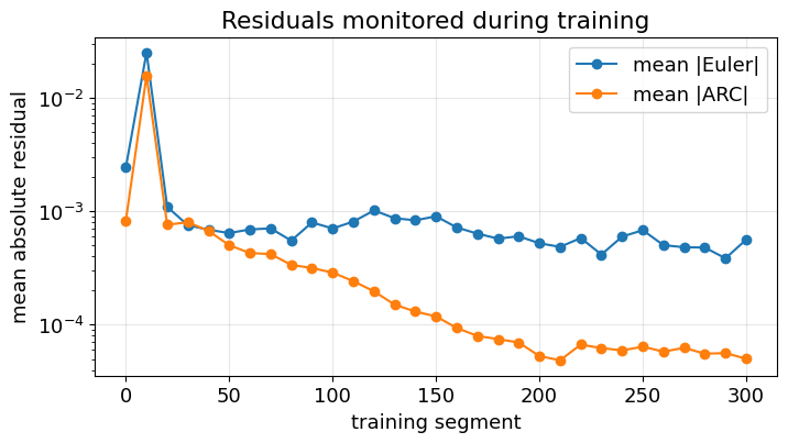
The mean absolute Euler error is a relative Euler wedge. For example, mean = 2e-3 means an average wedge of roughly 0.2 percent. The ARC error is a relative resource violation.
The next section adds two convergence checks: policy drift on a fixed holdout cloud and the zero-shock stochastic steady state.
def summarize_abs(x):
    x = np.asarray(x, dtype=np.float64).reshape(-1)
    return {
        "mean": float(np.mean(x)),
        "median": float(np.median(x)),
        "p95": float(np.quantile(x, 0.95)),
        "p99": float(np.quantile(x, 0.99)),
        "max": float(np.max(x)),
    }

def print_summary(name, values):
    s = summarize_abs(values)
    print(
        f"  {name:22s} "
        f"mean={s['mean']:.3e} ({100*s['mean']:.3f}%) | "
        f"median={s['median']:.3e} | p95={s['p95']:.3e} | "
        f"p99={s['p99']:.3e} | max={s['max']:.3e}"
    )

def simulated_evaluation_states(model, n_eval_tracks=64, burn_in=64, eval_length=256):
    X0 = sample_feasible_initial_states(n_eval_tracks)
    path, _ = simulate_path(X0, model, burn_in + eval_length)
    path = path[burn_in:]
    return tf.constant(path.reshape(-1, n_states), dtype=tf.float32)

def residual_report(label, X, model):
    loss, euler_res, arc_res, kp, lamb, c = compute_residuals(X, model)
    e_abs = np.abs(euler_res.numpy())
    a_abs = np.abs(arc_res.numpy())
    X_np = X.numpy() if isinstance(X, tf.Tensor) else np.asarray(X)
    kp_np = kp.numpy()

    print(f"\n{label}")
    print(f"  total loss              {float(loss.numpy()):.3e}")
    print_summary("|Euler relative|", e_abs)
    print_summary("|ARC relative|", a_abs)
    print(f"  log10 mean |Euler|      {np.log10(max(e_abs.mean(), 1e-30)): .3f}")
    print(f"  log10 mean |ARC|        {np.log10(max(a_abs.mean(), 1e-30)): .3f}")
    print(f"  capital in states       [{X_np[:, :N_COUNTRIES].min():.3f}, {X_np[:, :N_COUNTRIES].max():.3f}]")
    print(f"  capital chosen k'       [{kp_np.min():.3f}, {kp_np.max():.3f}]")

N_EVAL_EXOGENOUS = 8192 if RUN_MODE != "smoke" else 1024
N_EVAL_TRACKS = 64 if RUN_MODE != "smoke" else 8
EVAL_BURN_IN = 64 if RUN_MODE != "smoke" else 8
EVAL_LENGTH = 256 if RUN_MODE != "smoke" else 32

X_eval_exog = get_training_data_exogenous(N_EVAL_EXOGENOUS)
X_eval_sim = simulated_evaluation_states(model, N_EVAL_TRACKS, EVAL_BURN_IN, EVAL_LENGTH)

residual_report("Out-of-sample exogenous states", X_eval_exog, model)
residual_report("Out-of-sample simulated states", X_eval_sim, model)
Out-of-sample exogenous states
  total loss              1.135e-05
  |Euler relative|       mean=2.628e-03 (0.263%) | median=2.214e-03 | p95=6.366e-03 | p99=8.734e-03 | max=1.223e-02
  |ARC relative|         mean=5.580e-04 (0.056%) | median=3.860e-04 | p95=1.682e-03 | p99=2.279e-03 | max=3.327e-03
  log10 mean |Euler|      -2.580
  log10 mean |ARC|        -3.253
  capital in states       [0.550, 1.800]
  capital chosen k'       [0.551, 1.804]

Out-of-sample simulated states
  total loss              4.004e-06
  |Euler relative|       mean=1.675e-03 (0.167%) | median=1.619e-03 | p95=3.631e-03 | p99=4.492e-03 | max=5.781e-03
  |ARC relative|         mean=6.845e-05 (0.007%) | median=4.976e-05 | p95=2.037e-04 | p99=3.344e-04 | max=6.404e-04
  log10 mean |Euler|      -2.776
  log10 mean |ARC|        -4.165
  capital in states       [0.639, 1.571]
  capital chosen k'       [0.639, 1.571]
8. Time-invariance and zero-shock stochastic steady state¶
There are two different notions that are useful to keep separate.
First, the policy network has no calendar-time input, so a fixed set of weights always defines a time-homogeneous recursive policy. The nontrivial numerical question is whether the policy function has stopped changing as training proceeds. The notebook checks this by evaluating the policy on a fixed holdout cloud X_anchor and reporting the monitor-to-monitor policy drift.
Second, the stochastic steady state reported below is the fixed point of the learned stochastic policy when realized shocks are set to zero. It is not imposed during training. Starting from several dispersed feasible states, the notebook simulates the learned policy with zero shocks and checks whether all paths converge to a common economically meaningful point.
def final_time_invariance_report():
    """Summarize whether the learned policy has stabilized over training time."""
    print("\nTime-invariance / policy-stability diagnostic")

    # Same-state repeatability should be essentially machine precision because
    # the network has no dropout, no time input, and no random layer at inference.
    fp_1 = policy_fingerprint(X_anchor, model).numpy()
    fp_2 = policy_fingerprint(X_anchor, model).numpy()
    same_state_max = float(np.max(np.abs(fp_2 - fp_1)))
    print(f"  same-state repeatability, max abs difference = {same_state_max:.3e}")

    if len(history["policy_drift_rms"]) == 0:
        print("  no policy-drift history was recorded; increase NUM_SEGMENTS or lower MONITOR_EVERY")
        return

    last_rms = history["policy_drift_rms"][-1]
    last_max = history["policy_drift_max"][-1]
    print(f"  last monitor-to-monitor policy drift, rms = {last_rms:.3e}")
    print(f"  last monitor-to-monitor policy drift, max = {last_max:.3e}")
    print(f"  drift tolerances: rms <= {TIME_INVARIANCE_TOL_RMS:g}, max <= {TIME_INVARIANCE_TOL_MAX:g}")
    if last_rms <= TIME_INVARIANCE_TOL_RMS and last_max <= TIME_INVARIANCE_TOL_MAX:
        print("  PASS: policy drift is small on the fixed holdout cloud.")
    else:
        print("  WARNING: policy is still moving on the fixed holdout cloud. Train longer, reduce the learning rate, or increase the segment budget.")

def sample_zero_shock_start_states(n_tracks):
    """Deterministic dispersed starts for the zero-shock steady-state diagnostic."""
    local_rng = np.random.default_rng(SEED + 51031)
    log_k = local_rng.uniform(np.log(INITIAL_K_LOW), np.log(INITIAL_K_HIGH), size=(n_tracks, N_COUNTRIES))
    z0 = local_rng.uniform(INITIAL_Z_LOW, INITIAL_Z_HIGH, size=(n_tracks, N_COUNTRIES))
    return tf.constant(np.concatenate([np.exp(log_k), z0], axis=1).astype(np.float32), dtype=tf.float32)

def simulate_single_step_zero_shock(states, model):
    """One deterministic transition under the stochastic policy with realized shocks set to zero."""
    states = tf.convert_to_tensor(states, dtype=tf.float32)
    kp, _ = policy(states, model)
    z = states[:, N_COUNTRIES:]
    z_next = rho_z * z
    return tf.concat([kp, z_next], axis=1)

def scaled_transition_distance(x, x_next):
    """Scale-free distance between two consecutive zero-shock state arrays."""
    x = np.asarray(x, dtype=np.float64)
    x_next = np.asarray(x_next, dtype=np.float64)
    k = np.maximum(x[:, :N_COUNTRIES], EPS)
    kp = np.maximum(x_next[:, :N_COUNTRIES], EPS)
    z = x[:, N_COUNTRIES:]
    z_next = x_next[:, N_COUNTRIES:]
    d_k = np.max(np.abs(np.log(kp / k)))
    d_z = np.max(np.abs(z_next - z)) / max(INPUT_Z_SCALE, EPS)
    return float(max(d_k, d_z))

def compute_zero_shock_stochastic_steady_state(model):
    """Iterate the learned stochastic policy with realized shocks set to zero."""
    X = sample_zero_shock_start_states(ZERO_SHOCK_N_STARTS)
    distances = []
    converged = False

    for step in range(1, ZERO_SHOCK_MAX_STEPS + 1):
        X_next = simulate_single_step_zero_shock(X, model)
        X_np = X.numpy()
        X_next_np = X_next.numpy()
        if not np.all(np.isfinite(X_next_np)):
            print(f"  zero-shock iteration stopped at step {step}: non-finite state encountered")
            break
        dist = scaled_transition_distance(X_np, X_next_np)
        distances.append(dist)
        X = tf.constant(X_next_np.astype(np.float32), dtype=tf.float32)
        if dist <= ZERO_SHOCK_TOL:
            converged = True
            break

    return X, np.asarray(distances), step, converged

def pass_fail(condition):
    return "PASS" if bool(condition) else "FAIL"

def zero_shock_stochastic_steady_state_report(model):
    """Compute and economically sanity-check the zero-shock stochastic steady state."""
    if not RUN_ZERO_SHOCK_STEADY_STATE_CHECK:
        print("\nZero-shock stochastic steady-state diagnostic skipped.")
        return None

    print("\nZero-shock stochastic steady-state diagnostic")
    X_ss, distances, n_steps, converged = compute_zero_shock_stochastic_steady_state(model)
    X_np = X_ss.numpy()
    k = X_np[:, :N_COUNTRIES]
    z = X_np[:, N_COUNTRIES:]

    loss, euler_res, arc_res, kp, lamb, c = compute_residuals(X_ss, model)
    kp_np = kp.numpy()
    c_np = c.numpy()
    e_abs = np.abs(euler_res.numpy())
    a_abs = np.abs(arc_res.numpy())

    capital_fixed_error = float(np.max(np.abs(kp_np - k) / np.maximum(k, EPS)))
    max_abs_z = float(np.max(np.abs(z)))
    log_k_spread = float(np.max(np.std(np.log(np.maximum(k, EPS)), axis=0)))
    mean_k = k.mean(axis=0)
    rel_to_det = mean_k / K_REF - 1.0

    print(f"  zero-shock iteration steps       {n_steps}")
    print(f"  converged                       {converged}")
    if len(distances) > 0:
        print(f"  final scaled transition dist    {distances[-1]:.3e}")
    print(f"  deterministic reference k       {K_REF:.6f}")
    print(f"  mean stochastic steady-state k  {mean_k}")
    print(f"  relative k deviation from ref   {rel_to_det}")
    print(f"  max |k'(s_ss)-k_ss|/k_ss        {capital_fixed_error:.3e}")
    print(f"  max |z_ss|                      {max_abs_z:.3e}")
    print(f"  max cross-start std(log k)      {log_k_spread:.3e}")
    print(f"  min consumption at s_ss         {c_np.min():.3e}")
    print(f"  mean |Euler| at s_ss            {e_abs.mean():.3e}")
    print(f"  mean |ARC| at s_ss              {a_abs.mean():.3e}")

    checks = [
        ("finite state and policy", np.all(np.isfinite(X_np)) and np.all(np.isfinite(kp_np)) and np.all(np.isfinite(c_np))),
        ("positive capital", np.min(k) > 0.0),
        ("zero-shock iteration converged", converged),
        ("capital fixed point", capital_fixed_error <= ZERO_SHOCK_FIXED_POINT_TOL),
        ("productivity fixed point z approximately 0", max_abs_z <= ZERO_SHOCK_Z_TOL),
        ("starts converge to common point", log_k_spread <= ZERO_SHOCK_CROSS_TRACK_TOL),
        ("positive consumption", np.min(c_np) > 0.0),
        ("capital in broad economic range", np.min(k) >= SSS_K_MIN_OK * K_REF and np.max(k) <= SSS_K_MAX_OK * K_REF),
        ("Euler residual small at s_ss", e_abs.mean() <= SSS_MEAN_RESIDUAL_TOL),
        ("resource residual small at s_ss", a_abs.mean() <= SSS_MEAN_RESIDUAL_TOL),
    ]

    print("\n  Economic sanity checks")
    for label, ok in checks:
        print(f"    {pass_fail(ok):4s}  {label}")

    return {
        "X_ss": X_ss,
        "distances": distances,
        "converged": converged,
        "mean_k": mean_k,
        "relative_to_deterministic_k": rel_to_det,
        "capital_fixed_error": capital_fixed_error,
        "max_abs_z": max_abs_z,
        "mean_abs_euler": float(e_abs.mean()),
        "mean_abs_arc": float(a_abs.mean()),
    }

final_time_invariance_report()
zero_shock_result = zero_shock_stochastic_steady_state_report(model)
Time-invariance / policy-stability diagnostic
  same-state repeatability, max abs difference = 0.000e+00
  last monitor-to-monitor policy drift, rms = 1.190e-04
  last monitor-to-monitor policy drift, max = 5.373e-04
  drift tolerances: rms <= 0.001, max <= 0.01
  PASS: policy drift is small on the fixed holdout cloud.

Zero-shock stochastic steady-state diagnostic
  zero-shock iteration steps       750
  converged                       False
  final scaled transition dist    1.503e-04
  deterministic reference k       1.000000
  mean stochastic steady-state k  [1.0139934  0.99838674]
  relative k deviation from ref   [ 0.01399338 -0.00161326]
  max |k'(s_ss)-k_ss|/k_ss        1.501e-04
  max |z_ss|                      1.278e-18
  max cross-start std(log k)      7.267e-02
  min consumption at s_ss         4.586e-02
  mean |Euler| at s_ss            7.550e-04
  mean |ARC| at s_ss              3.445e-05

  Economic sanity checks
    PASS  finite state and policy
    PASS  positive capital
    FAIL  zero-shock iteration converged
    FAIL  capital fixed point
    PASS  productivity fixed point z approximately 0
    FAIL  starts converge to common point
    PASS  positive consumption
    PASS  capital in broad economic range
    PASS  Euler residual small at s_ss
    PASS  resource residual small at s_ss
9. Simple plots¶
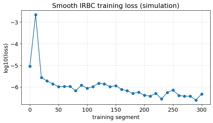
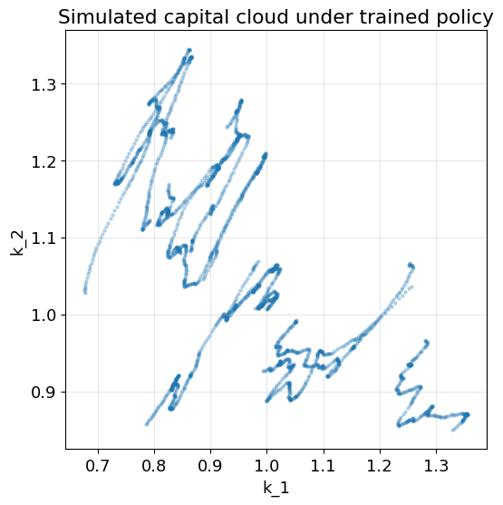
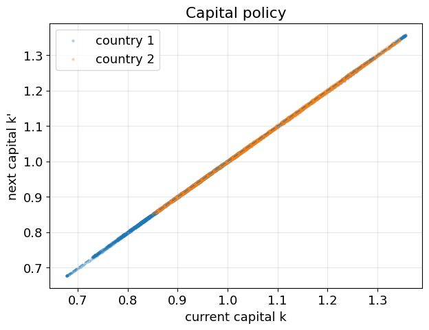
These plots are intentionally minimal. They show whether training is moving in the right direction and whether the simulated state cloud is well behaved.
if len(history.get("policy_drift_rms", [])) > 0:
    plt.figure(figsize=(8, 4))
    plt.plot(history["segment"], history["policy_drift_rms"], marker="o", label="RMS drift")
    plt.plot(history["segment"], history["policy_drift_max"], marker="o", label="max drift")
    plt.axhline(TIME_INVARIANCE_TOL_RMS, linestyle="--", label="RMS tolerance")
    plt.yscale("log")
    plt.xlabel("training segment")
    plt.ylabel("relative policy drift")
    plt.title("Policy-function drift on fixed holdout states")
    plt.legend()
    plt.grid(True, alpha=0.3)
    plt.show()

if isinstance(globals().get("zero_shock_result"), dict) and len(zero_shock_result["distances"]) > 0:
    plt.figure(figsize=(8, 4))
    plt.plot(np.arange(1, len(zero_shock_result["distances"]) + 1), zero_shock_result["distances"])
    plt.yscale("log")
    plt.xlabel("zero-shock iteration step")
    plt.ylabel("scaled transition distance")
    plt.title("Convergence to the zero-shock stochastic steady state")
    plt.grid(True, alpha=0.3)
    plt.show()

# Training curves.
plt.figure(figsize=(8, 4))
plt.plot(history["segment"], np.log10(np.maximum(history["loss"], 1e-30)), marker="o")
plt.xlabel("training segment")
plt.ylabel("log10(loss)")
plt.title(f"Smooth IRBC training loss ({SAMPLING_MODE})")
plt.grid(True, alpha=0.3)
plt.show()

plt.figure(figsize=(8, 4))
plt.plot(history["segment"], history["mean_abs_euler"], marker="o", label="mean |Euler|")
plt.plot(history["segment"], history["mean_abs_arc"], marker="o", label="mean |ARC|")
plt.yscale("log")
plt.xlabel("training segment")
plt.ylabel("mean absolute residual")
plt.title("Residuals monitored during training")
plt.legend()
plt.grid(True, alpha=0.3)
plt.show()

# A fresh simulated cloud under the trained policy.
X_cloud = simulated_evaluation_states(model, n_eval_tracks=10, burn_in=32, eval_length=256)
X_cloud_np = X_cloud.numpy()
kp_cloud, lambda_cloud = policy(X_cloud, model)

if N_COUNTRIES >= 2:
    plt.figure(figsize=(6, 6))
    plt.scatter(X_cloud_np[:, 0], X_cloud_np[:, 1], s=5, alpha=0.25)
    plt.xlabel("k_1")
    plt.ylabel("k_2")
    plt.title("Simulated capital cloud under trained policy")
    plt.grid(True, alpha=0.3)
    plt.show()

plt.figure(figsize=(7, 5))
for j in range(N_COUNTRIES):
    plt.scatter(X_cloud_np[:, j], kp_cloud.numpy()[:, j], s=5, alpha=0.25, label=f"country {j+1}")
lo = min(X_cloud_np[:, :N_COUNTRIES].min(), kp_cloud.numpy().min())
hi = max(X_cloud_np[:, :N_COUNTRIES].max(), kp_cloud.numpy().max())
plt.plot([lo, hi], [lo, hi], "--", alpha=0.6)
plt.xlabel("current capital k")
plt.ylabel("next capital k'")
plt.title("Capital policy")
plt.legend()
plt.grid(True, alpha=0.3)
plt.show()
10. How to change the training data¶
To use one long trajectory, set for example
N_TRAJECTORIES = 1
SIMULATION_LENGTH = 1024
To use several shorter trajectories, set for example
N_TRAJECTORIES = 10
SIMULATION_LENGTH = 256
To switch to exogenous sampling, set
SAMPLING_MODE = "exogenous"The optimizer is selected by OPTIMIZER_NAME, LEARNING_RATE, BATCH_SIZE, and PASSES_PER_SEGMENT in the first code cell.
The policy-stability check is controlled by TIME_INVARIANCE_ANCHOR_STATES, TIME_INVARIANCE_TOL_RMS, and TIME_INVARIANCE_TOL_MAX. The zero-shock stochastic steady-state check is controlled by RUN_ZERO_SHOCK_STEADY_STATE_CHECK, ZERO_SHOCK_N_STARTS, ZERO_SHOCK_MAX_STEPS, and ZERO_SHOCK_TOL.