Lecture 03, Notebook 05: Loss-Kernel Comparison on Brock–Mirman - Deep Learning for Solving and Estimating Dynamic Models in Economics and Finance

Course: Deep Learning for Solving and Estimating Dynamic Models in Economics and Finance
Script reference: §2.9 (choice of loss kernel: MSE / MAE / Huber / pinball / CVaR / log-cosh)
Notebook role: core
Author: Simon Scheidegger

RUN_MODE = "smoke"  # one of: "smoke", "teaching", "production"
SEED = 0

# Chapter-2 figure-output directory -- writes regenerated PNGs to slides/figures/.
import os
from pathlib import Path
FIG_DIR = Path('..') / 'slides' / 'figures'
FIG_DIR.mkdir(parents=True, exist_ok=True)
SAVE_FIGS = (RUN_MODE == 'production')  # only the production run regenerates the slide PNGs.
print(f"FIG_DIR = {FIG_DIR.resolve()},  SAVE_FIGS = {SAVE_FIGS}")

Brock-Mirman with Stochastic TFP: Loss Functions and Convergence¶

This notebook studies how the choice of training loss in a DEQN affects the economic convergence behaviour of the trained policy.

Two distinct objects are at play:

Training loss: the scalar that the optimizer minimises (MSE, MAE, Huber, Quantile pinball, CVaR, LogCosh, ...).
Economic loss: what we ultimately care about, the relative Euler equation error along a simulated path, which translates directly into a consumption-equivalent welfare loss.

These two are not the same. A loss that minimises the mean squared residual may leave a heavy right tail of residuals concentrated in rarely visited but economically consequential parts of the state space. We use the stochastic Brock-Mirman model with full depreciation, where the optimal savings rate is known in closed form,

s^\star \;=\; \alpha\beta,

(1)

to measure the discrepancy exactly. The same network is trained six times, once per loss kernel, with identical initialisation, optimizer, and training states (common random numbers). Only the reduction applied to the Euler residual differs.

Companion to: 02_Brock_Mirman_Uncertainty_DEQN.ipynb (same model, MSE only, partial depreciation). We switch to full depreciation here only to expose a closed-form benchmark.

1. Model: Stochastic Brock-Mirman (1972)¶

Production: $Y_t = e^{z_t} K_t^{\alpha}$
AR(1) for log TFP: $z_{t+1} = \rho\, z_t + \sigma\, \varepsilon_{t+1}$ , $\varepsilon \sim \mathcal{N}(0,1)$
Full depreciation, so capital evolves as $K_{t+1} = s_t Y_t$
Log utility, discount $\beta$
Euler equation: $\;1 \;=\; \beta\,\mathbb{E}_t\!\left[\dfrac{C_t}{C_{t+1}}\,\alpha e^{z_{t+1}} K_{t+1}^{\alpha-1}\right]$
Closed-form optimal savings rate: $s^\star = \alpha\beta$

The closed form is the reason for using $\delta=1$ : it gives an exact reference against which any learned policy can be measured, including a single-number consumption-equivalent welfare loss.

import numpy as np
import tensorflow as tf
from tensorflow import keras
import matplotlib.pyplot as plt
import time

plt.rcParams['font.size'] = 13
np.random.seed(SEED)
tf.random.set_seed(SEED)
tf.get_logger().setLevel('ERROR')   # silence harmless retracing warnings
print('TensorFlow', tf.__version__)

2026-04-27 11:20:53.910946: E external/local_xla/xla/stream_executor/cuda/cuda_fft.cc:477] Unable to register cuFFT factory: Attempting to register factory for plugin cuFFT when one has already been registered
WARNING: All log messages before absl::InitializeLog() is called are written to STDERR
E0000 00:00:1777281653.954935  588820 cuda_dnn.cc:8310] Unable to register cuDNN factory: Attempting to register factory for plugin cuDNN when one has already been registered
E0000 00:00:1777281653.967958  588820 cuda_blas.cc:1418] Unable to register cuBLAS factory: Attempting to register factory for plugin cuBLAS when one has already been registered
2026-04-27 11:20:54.005246: I tensorflow/core/platform/cpu_feature_guard.cc:210] This TensorFlow binary is optimized to use available CPU instructions in performance-critical operations.
To enable the following instructions: AVX2 FMA, in other operations, rebuild TensorFlow with the appropriate compiler flags.

TensorFlow 2.18.0

# Calibration (matches Day 2 stochastic BM, except delta=1).
alpha     = 0.36
beta      = 0.99
rho_tfp   = 0.9
sigma_tfp = 0.04

# Closed-form optimal savings rate.
s_star = alpha * beta
print(f'Optimal savings rate s* = alpha * beta = {s_star:.4f}')

# Steady-state log capital (deterministic, full depreciation).
K_ss  = (alpha * beta) ** (1.0 / (1.0 - alpha))
lk_ss = float(np.log(K_ss))
print(f'Deterministic steady state: K* = {K_ss:.4f},   log K* = {lk_ss:.4f}')

# Gauss-Hermite quadrature for the conditional expectation.
n_int = 5
_xi, _w = np.polynomial.hermite.hermgauss(n_int)
GH_NODES   = tf.constant(_xi * np.sqrt(2.0), dtype=tf.float32)   # innovations eps ~ N(0,1)
GH_WEIGHTS = tf.constant(_w / np.sqrt(np.pi), dtype=tf.float32)  # sum to 1

Optimal savings rate s* = alpha * beta = 0.3564
Deterministic steady state: K* = 0.1995,   log K* = -1.6120

2026-04-27 11:20:58.960693: E external/local_xla/xla/stream_executor/cuda/cuda_driver.cc:152] failed call to cuInit: INTERNAL: CUDA error: Failed call to cuInit: UNKNOWN ERROR (303)

2. Training-budget switch¶

All six losses share the same number of episodes; only the reduction kernel varies. Choose MODE based on what you want to do:

MODE	episodes / loss	total wall-clock (CPU)
`smoke`	300	~30 s
`teaching`	1500	~3 min
`production`	5000	~10 min

MODE = RUN_MODE  # aliased to the chapter-wide RUN_MODE switch in cell 1   # 'smoke' | 'teaching' | 'production'

if MODE == 'smoke':
    N_EPISODES, BATCH_SIZE, EVAL_EVERY = 300, 64, 25
elif MODE == 'teaching':
    N_EPISODES, BATCH_SIZE, EVAL_EVERY = 1500, 64, 50
elif MODE == 'production':
    N_EPISODES, BATCH_SIZE, EVAL_EVERY = 5000, 128, 100
else:
    raise ValueError(MODE)

print(f'MODE={MODE!r}: N_EPISODES={N_EPISODES}, BATCH_SIZE={BATCH_SIZE}, EVAL_EVERY={EVAL_EVERY}')

MODE='production': N_EPISODES=5000, BATCH_SIZE=128, EVAL_EVERY=100

3. Network¶

Identical 2x32 swish architecture across all six runs. Weights are saved once and reloaded for each loss kind so all runs start from the same point (this is what makes the comparison fair).

def make_network(seed=SEED):
    return keras.Sequential([
        keras.layers.Input(shape=(2,)),
        keras.layers.Dense(32, activation='swish',
            kernel_initializer=keras.initializers.GlorotUniform(seed=seed)),
        keras.layers.Dense(32, activation='swish',
            kernel_initializer=keras.initializers.GlorotUniform(seed=seed+1)),
        keras.layers.Dense(1,  activation='sigmoid',
            kernel_initializer=keras.initializers.GlorotUniform(seed=seed+2)),
    ])

_init_nn = make_network(seed=SEED)
INIT_WEIGHTS = _init_nn.get_weights()
_init_nn.summary()

4. Euler residual and ground truth¶

We work with the relative residual

r(k_t,z_t) \;=\; \beta\,\mathbb{E}_t\!\Big[\tfrac{C_t}{C_{t+1}}\, \alpha e^{z_{t+1}} K_{t+1}^{\alpha-1}\Big] - 1,

(2)

evaluated by Gauss-Hermite quadrature. Every loss kernel below is a different reduction of $r$ to a scalar; the residual itself is identical across runs.

@tf.function
def euler_residual(state, nn):
    '''Return relative Euler residual r at each state. state shape (B, 2).
       Columns: (z_t, log K_t).  s_t comes from the network, sigmoid -> (0,1).'''
    z_t  = state[:, 0:1]
    lk_t = state[:, 1:2]
    Z_t  = tf.exp(z_t)
    K_t  = tf.exp(lk_t)
    Y_t  = Z_t * K_t**alpha
    s_t  = nn(state)
    K_tp1 = s_t * Y_t                       # delta = 1
    C_t   = (1.0 - s_t) * Y_t
    lk_tp1 = tf.math.log(K_tp1)

    expectation = tf.zeros_like(z_t)
    for q in range(n_int):
        eps_q  = GH_NODES[q]                # already includes sqrt(2)
        z_tp1  = rho_tfp * z_t + sigma_tfp * eps_q
        Z_tp1  = tf.exp(z_tp1)
        state_tp1 = tf.concat([z_tp1, lk_tp1], axis=1)
        s_tp1  = nn(state_tp1)
        Y_tp1  = Z_tp1 * K_tp1**alpha
        C_tp1  = (1.0 - s_tp1) * Y_tp1
        r_tp1  = alpha * Z_tp1 * K_tp1**(alpha - 1.0)
        integrand = (C_t / C_tp1) * r_tp1
        expectation = expectation + GH_WEIGHTS[q] * integrand
    return beta * expectation - 1.0

5. The six loss kernels¶

All operate on the same vector $r \in \mathbb{R}^B$ produced by the cell above. Only the reduction differs:

Kernel	Formula	Emphasis
MSE	$\frac1B\sum r^2$	mean of squared residuals (canonical DEQN choice)
MAE	$\frac1B\sum \|r\|$	median, robust to outliers; gradient magnitude is constant, so progress at small residuals stalls
Huber	quadratic for $\|r\| \le \delta$ , linear above	smooth hybrid of MSE / MAE, but the quadratic-to-linear switch at $\|r\|{=}\delta$ is a kink in the gradient
Quantile	pinball at $\tau{=}0.9$ : $\max(\tau r,(\tau{-}1)r)$	trains the upper $\tau$ -quantile of $r$ specifically
CVaR	mean of top $(1{-}\alpha){=}10\%$ of $\|r\|$	tail mean - explicitly trains the bad regions
LogCosh	$\frac1B\sum \log\cosh(r)$	smooth ( $C^\infty$ ) hybrid: $\frac{1}{2}r^2$ near zero, $\|r\|-\log 2$ in the tails - quadratic curvature where it helps fine convergence, linear asymptote where it tames outliers, no kink anywhere

def make_loss(kind, **kw):
    '''Return a function residuals -> scalar loss. All operate on the same r.'''
    if kind == 'MSE':
        return lambda r: tf.reduce_mean(r**2)
    if kind == 'MAE':
        return lambda r: tf.reduce_mean(tf.abs(r))
    if kind == 'Huber':
        delta = tf.constant(kw.get('delta', 1e-2), dtype=tf.float32)
        def huber(r):
            ar = tf.abs(r)
            quad = 0.5 * r**2
            lin  = delta * (ar - 0.5 * delta)
            return tf.reduce_mean(tf.where(ar <= delta, quad, lin))
        return huber
    if kind == 'Quantile':
        tau = tf.constant(kw.get('tau', 0.9), dtype=tf.float32)
        def pinball(r):
            return tf.reduce_mean(tf.maximum(tau * r, (tau - 1.0) * r))
        return pinball
    if kind == 'CVaR':
        alpha_cvar = float(kw.get('alpha', 0.9))
        def cvar(r):
            abs_r = tf.abs(tf.reshape(r, [-1]))
            n = tf.shape(abs_r)[0]
            k = tf.maximum(tf.cast(tf.cast(n, tf.float32) * (1.0 - alpha_cvar), tf.int32), 1)
            top_k_vals, _ = tf.math.top_k(abs_r, k=k)
            return tf.reduce_mean(top_k_vals)
        return cvar
    if kind == 'LogCosh':
        return lambda r: tf.reduce_mean(tf.math.log(tf.math.cosh(r)))
    raise ValueError(kind)

LOSS_KINDS = ['MSE', 'MAE', 'Huber', 'Quantile', 'CVaR', 'LogCosh']

6. Common random numbers¶

We pre-generate every training batch once: each loss run sees exactly the same sequence of training states. The only difference between runs is the reduction applied to the residual. This is what makes the comparison fair. Evaluation is done on a fixed $(z, \log K)$ grid spanning the ergodic support.

rng  = np.random.default_rng(SEED)   # SEED from cell 2

# Pre-generate every training batch (same for all losses).
TOTAL = N_EPISODES * BATCH_SIZE
z_sd_ergodic = sigma_tfp / np.sqrt(1.0 - rho_tfp**2)
z_train  = rng.normal(loc=0.0, scale=z_sd_ergodic, size=TOTAL).astype(np.float32)
lk_train = rng.uniform(low=lk_ss - 0.5, high=lk_ss + 0.5, size=TOTAL).astype(np.float32)
TRAIN_STATES = tf.constant(np.stack([z_train, lk_train], axis=1))

# Evaluation grid: 21 x 21 in (z, log K) covering ~3 sigma of the ergodic dist.
z_eval_grid  = np.linspace(-3.0 * z_sd_ergodic, 3.0 * z_sd_ergodic, 21).astype(np.float32)
lk_eval_grid = np.linspace(lk_ss - 0.4, lk_ss + 0.4, 21).astype(np.float32)
ZZ, LK = np.meshgrid(z_eval_grid, lk_eval_grid, indexing='ij')
EVAL_STATES = tf.constant(np.stack([ZZ.ravel(), LK.ravel()], axis=1))

# Welfare-comparison shocks: one fixed sequence used for every kind.
T_PATH = 2000
PATH_INNOVATIONS = tf.constant(rng.normal(size=T_PATH).astype(np.float32))

print(f'Training points pre-generated: {TOTAL}')
print(f'Eval grid: {EVAL_STATES.shape[0]} states')
print(f'Welfare path length: {T_PATH}')

Training points pre-generated: 640000
Eval grid: 441 states
Welfare path length: 2000

7. Training rig¶

One JIT-compiled train_step per loss kind (the loss function is captured in the closure, so each kind compiles its own graph). Per-episode logging evaluates the economic metric (relative Euler error on the eval grid) every EVAL_EVERY steps.

def fresh_nn():
    nn = make_network(seed=SEED)
    nn.set_weights(INIT_WEIGHTS)
    return nn

def make_train_step(loss_fn):
    @tf.function
    def step(batch_states, nn, optimizer):
        with tf.GradientTape() as tape:
            r = euler_residual(batch_states, nn)
            loss = loss_fn(r)
        grads = tape.gradient(loss, nn.trainable_variables)
        optimizer.apply_gradients(zip(grads, nn.trainable_variables))
        return loss
    return step

def run_one_loss(kind, **kw):
    nn        = fresh_nn()
    optimizer = tf.keras.optimizers.Adam(learning_rate=1e-3)
    loss_fn   = make_loss(kind, **kw)
    step      = make_train_step(loss_fn)

    log_train_loss, log_mean, log_p90, log_p99 = [], [], [], []
    eval_eps = []

    t0 = time.time()
    for e in range(N_EPISODES):
        batch = TRAIN_STATES[e * BATCH_SIZE : (e + 1) * BATCH_SIZE]
        loss  = float(step(batch, nn, optimizer))
        if (e % EVAL_EVERY) == 0 or e == N_EPISODES - 1:
            r_eval = euler_residual(EVAL_STATES, nn).numpy().ravel()
            ar     = np.abs(r_eval)
            log_train_loss.append(loss)
            log_mean.append(ar.mean())
            log_p90.append(np.quantile(ar, 0.90))
            log_p99.append(np.quantile(ar, 0.99))
            eval_eps.append(e)
    elapsed = time.time() - t0
    return dict(kind=kind, nn=nn,
                eval_eps=np.array(eval_eps),
                train_loss=np.array(log_train_loss),
                eval_mean=np.array(log_mean),
                eval_p90=np.array(log_p90),
                eval_p99=np.array(log_p99),
                elapsed=elapsed)

results = {}
for kind in LOSS_KINDS:
    print(f'Training with {kind:<9s} loss ...', end=' ', flush=True)
    results[kind] = run_one_loss(kind)
    r = results[kind]
    print(f'done in {r["elapsed"]:5.1f}s | final mean |r|={r["eval_mean"][-1]:.2e}, p99|r|={r["eval_p99"][-1]:.2e}')

Training with MSE       loss ...

done in  18.5s | final mean |r|=1.37e-04, p99|r|=4.03e-04
Training with MAE       loss ...

done in  21.4s | final mean |r|=2.51e-03, p99|r|=2.91e-03
Training with Huber     loss ...

done in  18.7s | final mean |r|=3.95e-04, p99|r|=6.24e-04
Training with Quantile  loss ...

done in  18.0s | final mean |r|=1.16e-03, p99|r|=2.29e-03
Training with CVaR      loss ...

done in  19.6s | final mean |r|=4.41e-04, p99|r|=8.34e-04
Training with LogCosh   loss ...

done in  17.6s | final mean |r|=1.25e-04, p99|r|=3.89e-04

8. Convergence of the economic metric¶

Three panels: the mean, $p_{90}$ , and $p_{99}$ of the absolute relative Euler error on the evaluation grid, plotted against the training episode. All curves are on a log scale, so vertical distance is multiplicative.

Reproducing the published figure. The PNG that ships with the slides (slides/figures/loss_kernel_convergence.png) and the script (lecture_script/fig/loss_kernel_convergence.png) was produced under RUN_MODE = 'production' (5 000 episodes / kernel). The default RUN_MODE = 'teaching' (1 500 episodes / kernel, formerly named classroom) trains in roughly three minutes on a CPU and is good enough to see the qualitative ordering, but the curves will not match the published figure pixel-for-pixel.

fig, axes = plt.subplots(1, 3, figsize=(15.5, 4.5))
for kind in LOSS_KINDS:
    r = results[kind]
    axes[0].semilogy(r['eval_eps'], r['eval_mean'], label=kind)
    axes[1].semilogy(r['eval_eps'], r['eval_p90'],  label=kind)
    axes[2].semilogy(r['eval_eps'], r['eval_p99'],  label=kind)
for ax, t in zip(axes, ['mean |r|', 'p90 |r|', 'p99 |r|']):
    ax.set_xlabel('Training episode'); ax.set_ylabel(t)
    ax.set_title(f'Eval-grid {t}'); ax.grid(True, which='both', alpha=0.3)
axes[0].legend(fontsize=10, loc='best')
plt.tight_layout()
if SAVE_FIGS:
    fig.savefig(FIG_DIR / 'loss_kernel_convergence.png',
                dpi=150, bbox_inches='tight')
plt.show()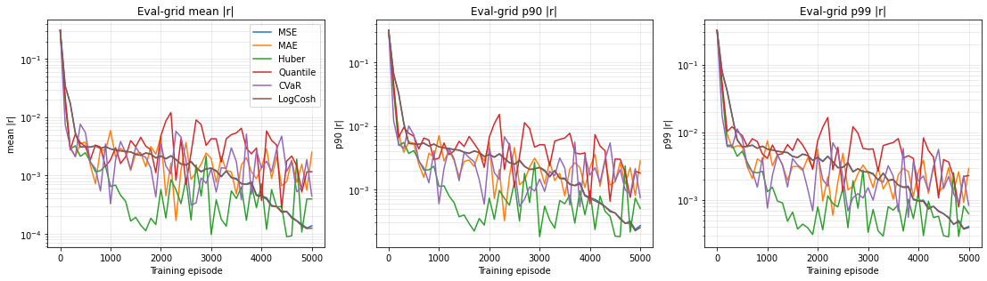

9. Final economic metric: along an actual simulated path¶

After training, we forward-simulate each learned policy (and the closed-form optimum $s^\star$ ) under the same fixed innovation sequence (PATH_INNOVATIONS). At every state visited along the path we compute the absolute relative Euler residual; we also compute the consumption- equivalent welfare loss of the learned policy versus $s^\star$ ,

\lambda \;=\; 1 - \exp\!\Big((1-\beta)\,(U_{\text{learned}} - U^\star)\Big),

(3)

the fraction of consumption that the agent would forgo to switch from the learned policy to the optimum.

@tf.function(reduce_retracing=True)
def simulate_with_policy(policy_fn, T, z0, lk0, innovations):
    log_c = tf.TensorArray(tf.float32, size=T)
    states_hist = tf.TensorArray(tf.float32, size=T, element_shape=[2])
    z, lk = z0, lk0
    for t in tf.range(T):
        state_t = tf.stack([[z, lk]], axis=0)
        states_hist = states_hist.write(t, state_t[0])
        s_t = policy_fn(state_t)[0, 0]
        Z_t = tf.exp(z); K_t = tf.exp(lk)
        Y_t = Z_t * K_t**alpha
        c_t = (1.0 - s_t) * Y_t
        log_c = log_c.write(t, tf.math.log(c_t))
        K_tp1 = s_t * Y_t
        lk = tf.math.log(K_tp1)
        z = rho_tfp * z + sigma_tfp * innovations[t]
    return log_c.stack(), states_hist.stack()

def utility(log_c, beta_=beta):
    T = tf.shape(log_c)[0]
    discount = beta_ ** tf.cast(tf.range(T), tf.float32)
    return tf.reduce_sum(discount * log_c)

# Optimal policy: constant savings rate s*
s_star_tf = tf.constant(s_star, dtype=tf.float32)
def s_opt(state): return tf.fill((tf.shape(state)[0], 1), s_star_tf)

z0_tf  = tf.constant(0.0, dtype=tf.float32)
lk0_tf = tf.constant(lk_ss, dtype=tf.float32)
log_c_opt, _ = simulate_with_policy(s_opt, T_PATH, z0_tf, lk0_tf, PATH_INNOVATIONS)
U_opt = utility(log_c_opt)

summary_rows = []
for kind in LOSS_KINDS:
    nn = results[kind]['nn']
    log_c, states_hist = simulate_with_policy(lambda s: nn(s), T_PATH,
                                              z0_tf, lk0_tf, PATH_INNOVATIONS)
    U = utility(log_c)
    lam = 1.0 - float(tf.exp((1.0 - beta) * (U - U_opt)).numpy())  # CE welfare loss
    # Euler residual at every state actually visited
    ar_path = np.abs(euler_residual(states_hist, nn).numpy().ravel())
    summary_rows.append((kind, ar_path.mean(), np.median(ar_path),
                         np.quantile(ar_path, 0.9), np.quantile(ar_path, 0.99),
                         ar_path.max(), lam))
    results[kind]['path_residuals'] = ar_path
    results[kind]['CE_loss'] = lam

print(f'Path length T = {T_PATH}; closed-form s* = {s_star:.4f}')
print()
print(f'{"Loss":<10}{"mean |r|":>12}{"p50":>12}{"p90":>12}{"p99":>12}{"max":>12}{"CE loss":>12}')
print('-' * 82)
for k, m, p50, p90, p99, mx, lam in summary_rows:
    print(f'{k:<10}{m:>12.2e}{p50:>12.2e}{p90:>12.2e}{p99:>12.2e}{mx:>12.2e}{lam*100:>11.4f}%')

Path length T = 2000; closed-form s* = 0.3564

Loss          mean |r|         p50         p90         p99         max     CE loss
----------------------------------------------------------------------------------
MSE           1.59e-04    1.63e-04    2.63e-04    2.98e-04    3.57e-04     0.0000%
MAE           2.48e-03    2.47e-03    2.73e-03    2.87e-03    2.96e-03     0.0003%
Huber         3.80e-04    3.74e-04    4.83e-04    5.32e-04    6.46e-04     0.0000%
Quantile      1.01e-03    9.87e-04    1.17e-03    1.64e-03    2.30e-03     0.0000%
CVaR          4.35e-04    4.38e-04    6.94e-04    7.95e-04    8.79e-04     0.0000%
LogCosh       1.37e-04    1.39e-04    2.43e-04    2.80e-04    3.42e-04    -0.0000%

fig, ax = plt.subplots(1, 1, figsize=(9, 5))
bins = np.logspace(-7, 0, 60)
for kind in LOSS_KINDS:
    ax.hist(results[kind]['path_residuals'], bins=bins, histtype='step',
            linewidth=1.6, label=kind)
ax.set_xscale('log'); ax.set_xlabel('|r|  (relative Euler residual along simulated path)')
ax.set_ylabel('count'); ax.set_title('Distribution of path Euler residuals by training loss')
ax.legend(fontsize=10); ax.grid(True, which='both', alpha=0.3)
plt.tight_layout()
if SAVE_FIGS:
    fig.savefig(FIG_DIR / 'loss_kernel_path_residuals.png',
                dpi=150, bbox_inches='tight')
plt.show()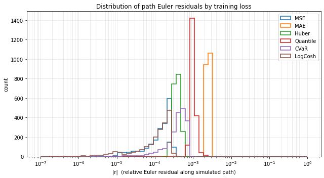

10. Do all six policies reach the same stochastic steady state?¶

A natural fairness question: each kernel produces a slightly different policy, so each one will simulate a slightly different ergodic distribution of capital under the same shocks. The closed-form optimum sits at $s^\star = \alpha\beta$ exactly; if a kernel converges to a near-optimal policy, the resulting stochastic steady state should be near-identical to the optimum’s. The block below verifies this directly: each policy is forward-simulated under PATH_INNOVATIONS for T_PATH = 2000 periods, the first 200 periods are dropped as burn-in, and the remaining ergodic window is used to compute the mean and standard deviation of $\log K_t$ , of the realised savings rate $s_t$ , and of output $e^{z_t} K_t^\alpha$ . All six rows should be close to the OPTIMAL row; differences quantify how much each kernel’s residual error perturbs the simulated economy.

import numpy as np

T_BURN = 200
print(f'Stochastic steady-state moments  (T={T_PATH}, dropping first {T_BURN} periods):')
print()
print(f'{"Policy":<10}{"E[log K]":>12}{"Std[log K]":>12}{"E[s_t]":>12}{"Std[s_t]":>12}{"E[Y_t]":>12}')
print('-' * 70)

# OPTIMAL: s* constant
_, st = simulate_with_policy(s_opt, T_PATH, z0_tf, lk0_tf, PATH_INNOVATIONS)
st_np = st.numpy()
z   = st_np[T_BURN:, 0]
lk  = st_np[T_BURN:, 1]
s_t = np.full_like(lk, s_star)
Y_t = np.exp(z) * np.exp(lk) ** alpha
print(f'{"OPTIMAL":<10}{lk.mean():>12.4f}{lk.std():>12.4f}{s_t.mean():>12.4f}{s_t.std():>12.4f}{Y_t.mean():>12.4f}')

ss_rows = []
for kind in LOSS_KINDS:
    nn = results[kind]['nn']
    _, st = simulate_with_policy(lambda s: nn(s), T_PATH, z0_tf, lk0_tf, PATH_INNOVATIONS)
    st_np = st.numpy()
    z   = st_np[T_BURN:, 0]
    lk  = st_np[T_BURN:, 1]
    s_t = nn(tf.constant(st_np[T_BURN:])).numpy().ravel()
    Y_t = np.exp(z) * np.exp(lk) ** alpha
    ss_rows.append((kind, lk.mean(), lk.std(), s_t.mean(), s_t.std(), Y_t.mean()))
    print(f'{kind:<10}{lk.mean():>12.4f}{lk.std():>12.4f}{s_t.mean():>12.4f}{s_t.std():>12.4f}{Y_t.mean():>12.4f}')

print()
print('Reading: column E[s_t] should be close to alpha * beta = ' f'{s_star:.4f}.')
print('         Std[s_t] is the spread of the learned savings rate around the optimum;')
print('         it is exactly zero for the closed-form optimum and grows with residual error.')

Stochastic steady-state moments  (T=2000, dropping first 200 periods):

Policy        E[log K]  Std[log K]      E[s_t]    Std[s_t]      E[Y_t]
----------------------------------------------------------------------
OPTIMAL        -1.6210      0.1288      0.3564      0.0000      0.5594

MSE            -1.6212      0.1287      0.3563      0.0000      0.5594

MAE            -1.6171      0.1285      0.3573      0.0001      0.5602

Huber          -1.6216      0.1287      0.3563      0.0000      0.5593

Quantile       -1.6194      0.1289      0.3568      0.0001      0.5597

CVaR           -1.6216      0.1285      0.3562      0.0001      0.5593

LogCosh        -1.6212      0.1287      0.3564      0.0000      0.5594

Reading: column E[s_t] should be close to alpha * beta = 0.3564.
         Std[s_t] is the spread of the learned savings rate around the optimum;
         it is exactly zero for the closed-form optimum and grows with residual error.

11. Where in the state space does each loss leave error?¶

Heat-map of $|s_{\text{learned}}(z, \log K) - s^\star|$ on the evaluation grid. Bright spots flag regions where the learned policy disagrees with the closed-form optimum.

n = len(LOSS_KINDS)
fig, axes = plt.subplots(1, n, figsize=(2.6 * n, 3.0), sharex=True, sharey=True)
err_maps, vmax = {}, 0.0
for kind in LOSS_KINDS:
    nn = results[kind]['nn']
    s_pred = nn(EVAL_STATES).numpy().ravel().reshape(ZZ.shape)
    err_maps[kind] = np.abs(s_pred - s_star)
    vmax = max(vmax, err_maps[kind].max())
for ax, kind in zip(axes, LOSS_KINDS):
    im = ax.imshow(err_maps[kind].T, origin='lower',
                   extent=[z_eval_grid[0], z_eval_grid[-1], lk_eval_grid[0], lk_eval_grid[-1]],
                   aspect='auto', vmin=0, vmax=vmax, cmap='viridis')
    ax.set_title(f'{kind}\nmax={err_maps[kind].max():.1e}', fontsize=10)
    ax.set_xlabel('z'); ax.set_ylabel('log K')
fig.colorbar(im, ax=axes.tolist(), shrink=0.85, label='|s - s*|')
if SAVE_FIGS:
    fig.savefig(FIG_DIR / 'loss_kernel_state_error.png',
                dpi=150, bbox_inches='tight')
plt.show()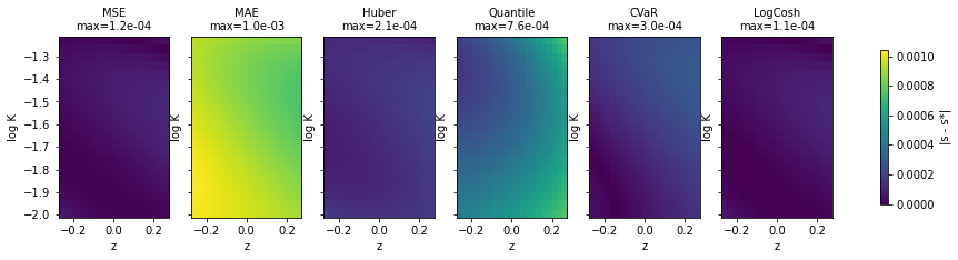

12. Discussion¶

Several patterns typically emerge from the run above.

MSE drives the bulk down fast but its quadratic gradient also amplifies any outlier residual; in practice this means MSE training curves look smooth on average but can have visible jitter when an unusual mini-batch lands.

MAE stalls at a finite floor. The gradient of $|r|$ has constant magnitude (its sign), so once residuals are small, the optimizer takes the same step regardless of how close to zero it already is. The result is a clean log-curve that levels off and refuses to drop further. This is exactly the textbook MAE pathology, made visible here on a smooth model.

Huber is robust but kinked. It mimics MSE for $|r| \le \delta$ and MAE for $|r| > \delta$ , so it inherits MSE’s fine-convergence behaviour in the bulk and MAE’s outlier robustness. The downside: the gradient has a jump at $|r|=\delta$ , which can introduce small training-loop oscillations as residuals migrate across that threshold.

Quantile and CVaR explicitly target the tail. They typically deliver the narrowest spread between mean and max residual, at a small cost in mean (Quantile pays the most because it ignores most of the distribution by construction). When the worst-case policy quality matters, this is the right trade.

LogCosh tends to converge most smoothly of the six. It is the unique kernel here that is both $C^\infty$ everywhere and combines the two desirable asymptotic regimes: $\log\cosh(r) \approx \tfrac{1}{2} r^2$ for small $|r|$ (so it inherits MSE’s fine-grained convergence near zero) and $\log\cosh(r) \approx |r| - \log 2$ for large $|r|$ (so its gradient saturates at $\pm 1$ , which tames outliers like MAE). Crucially, the transition between the two regimes is smooth, with no kink as in Huber. Visually, the log-cosh convergence curve is essentially monotone with no spikes; numerically, it tracks MSE in the bulk and matches Huber on the tail. For most practical DEQN settings, log-cosh is therefore the lowest-risk choice when the modeller is unsure how rough or peaked the residual distribution will be in advance, and that is why it deserves a closer look beyond the usual MSE / Huber pair.

The CE-welfare-loss ranking is not the same as the training-loss ranking. Lifetime utility under log preferences is sensitive to outlier consumption realisations; a tail-aware loss can deliver lower welfare loss even when its mean Euler residual is larger.

Take-away. We do not actually care about MSE. We care about the behaviour of the policy along simulated equilibrium paths, in consumption-equivalent welfare terms. The training loss is just an instrument; choosing it with that hierarchy in mind is part of the modelling decision. For models with sharp non-linearities or rare-event regions (occasionally binding constraints, tipping risks, fat-tailed shocks), tail-aware kernels pay off. For smooth, well-behaved problems the difference is mostly cosmetic and MSE is fine - but log-cosh is rarely a bad default.

Practical guidance.

Default to MSE unless you have a reason not to. LogCosh is a near-equivalent drop-in that is more forgiving when residuals are heavy-tailed; it is the lowest-risk choice when in doubt.
Use Huber when training is unstable on a few outlier states (a common symptom: occasional loss spikes that re-converge slowly). Note that the kink at $|r|{=}\delta$ can itself induce mild oscillation.
Use Quantile $\tau{=}0.9$ or CVaR $\alpha{=}0.9$ when the worst-case policy quality matters: occasionally binding constraints, rare-but-consequential states, regulatory back-tests.
Avoid MAE as the sole training loss for fine-grained convergence: its constant gradient magnitude prevents the optimizer from making smaller steps as residuals shrink, and it stalls at a noise-floor that is much higher than what MSE / log-cosh / Huber attain at the same training budget.
Always evaluate on the economic metric, the relative Euler residual along simulated paths, not on the training loss itself.

Further exercises.

Sweep the quantile level $\tau \in \{0.5, 0.9, 0.99\}$ and watch the bias-variance trade-off shift.
Combine losses: $\ell = \ell_{\text{MSE}} + \eta\, \ell_{\text{CVaR}}$ with $\eta$ small. This typically gives the cleanest convergence both in the bulk and the tail.
Re-run with $\delta=0.1$ (the partial-depreciation Day-2 calibration). The closed-form benchmark is no longer available, but the relative ranking of losses on path Euler residuals should be qualitatively the same.
Repeat the experiment with the Day-3 IRBC notebook; tail-aware losses matter more when the state dimension grows.