Lecture 03, Notebook 01: Deterministic Brock–Mirman DEQN - Deep Learning for Solving and Estimating Dynamic Models in Economics and Finance

Course: Deep Learning for Solving and Estimating Dynamic Models in Economics and Finance
Script reference: §2.4 (deterministic Brock–Mirman benchmark), §2.5 (hard/soft constraint split)
Notebook role: core
Author: Simon Scheidegger

RUN_MODE = "smoke"  # one of: "smoke", "teaching", "production"
SEED = 0

# Chapter-wide RUN_MODE budget helper -- maps RUN_MODE to a training budget.
_BUDGET = {
    "smoke":      201,    # ~10 s, sanity check only
    "teaching":  2001,    # ~1 min CPU, default for live class
    "production": 10001,  # ~5 min CPU, publication run
}
NUM_EPISODES = _BUDGET[RUN_MODE]
print(f"RUN_MODE={RUN_MODE!r}: NUM_EPISODES={NUM_EPISODES}")

Simple Introduction to Deep Equilibrium Nets¶

Notebook 1: no uncertainty and exogenous sampling of states¶

Purpose of the notebook and economic model¶

The notebook should serve as a simple introduction to Deep Equilibrium Nets, a deep learning based method introduced in Azinovic et al. (2022).
To focus on the method, we are going to solve a simple optimal growth model with one representative agent, a simplified version of Brock and Mirman (1972).

The planner aims to maximize her time-separable life time utility subject to her budget constraint:

\begin{align*} &\max_{\left\{c_{t}\right\}_{t=0}^{\infty}} \sum_{t=0}^{\infty} \beta^{t} \ln\left(C_{t}\right) \tag{1} \\ \text{s.t.} \quad & K_{t+1} + C_{t} = Y_t + (1 - \delta) K_t \tag{2} \end{align*}

where $Y_t = K_{t} ^ \alpha$ .

When we assume full depreciation, i.e. $\delta=1$ , this particular problem has an analytical solution:

\begin{align} K_{t+1} = \beta \alpha K_{t}^{\alpha} \end{align}

(3)

We can numerically solve the above planner’s problem by using any global solution algorithm such as the value function iteration or the time iteration collocation.
However in this notebook, we demonstrate how the recursive equilibrium can be directly approximated by the deep neural net following Azinovic et al. (2022).

Following Azinovic et al. (2022) the idea is to express the equilibrium conditions as a set of equations, which need to be satisfied in equilibrium and which characterize the optimal policies. Having such a set of equations and a candidate policy function, the extent to which the equations are satisfied can serve as a measure for the accuracy of the candidate policy funcion.
The above problem can be formulated recursively, where the Bellman equation is given by

\begin{align*} V(K_t) &= \max_{K_{t+1}} \ln\left(C_{t}\right)+\beta V(K_{t+1}) \tag{4} \\ \text{subject to: }C_t &= Y_t + (1 - \delta) K_t - K_{t+1} \tag{5} \end{align*}

Plugging in the budget constraint, we obtain

\begin{align} V(K_t) &= \max_{K_{t+1}} \ln\left(Y_t + (1 - \delta) K_t - K_{t+1}\right)+\beta V(K_{t+1}). \end{align}

(6)

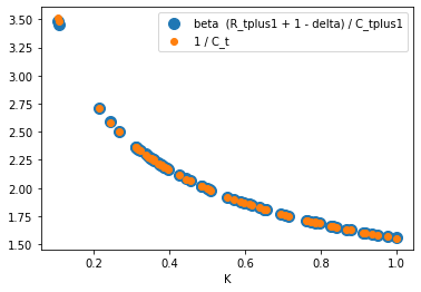
$K_t$ denotes the state of the economy and $K_{t+1} = f(K_t)$ denotes the policy. We are interested in approximating the policy $f(\cdot)$ with a neural network $\mathcal{N}(\cdot)$ , such that $\mathcal{N}(K_t) \approx f(K_t) = K_{t+1}$ .
Taking the first order condition with respect to $K_{t+1}$ , we obtain

\begin{align} 0 &= -\frac{1}{\underbrace{Y_t + (1 - \delta) K_t - K_{t+1}}_{=C_t}}+\beta \frac{d V(K_{t+1})}{d K_{t+1}} \end{align}

(7)

Applying the Envelope theorem, we obtain

\begin{align*} \frac{d V(K_{t})}{d K_{t}} &= \frac{d}{d K_{t}}\ln\left(\underbrace{Y_t + (1 - \delta) K_t - K_{t+1}}_{=C_t}\right) \tag{8} \\ &= \frac{1}{C_t}\left(\frac{dY_t}{dK_t} + (1 - \delta)\right) \tag{9} \\ &= \frac{1}{C_t}\left(\underbrace{\alpha K_{t}^{\alpha - 1}}_{=:r_t} + (1 - \delta)\right) \tag{10} \\ &= \frac{1}{C_t}\left(r_t + 1 - \delta\right). \tag{11} \end{align*}

Applying this result to replace $\frac{d V(K_{t+1})}{d K_{t+1}}$ in the first order condition, we obtain

\begin{align} 0 &= -\frac{1}{C_t} + \beta \frac{1}{C_{t+1}}\left(1 - \delta + r_{t+1}\right) \end{align}

(12)

where

\begin{align*} r_{t+1} &= \alpha K_{t+1}^{\alpha - 1} \tag{13} \\ C_t &= Y_t + (1 - \delta) K_t - K_{t+1} \tag{14} \\ C_{t+1} &= Y_{t+1} + (1 - \delta) K_{t+1} - K_{t+2}. \tag{15} \end{align*}

Our goal is now to find a policy function $f(\cdot)$ , such that this equation is fullfilled for $K_{t+1}= f(K_t)$ and $K_{t+2}= f(K_{t+1})$ .
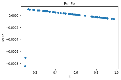
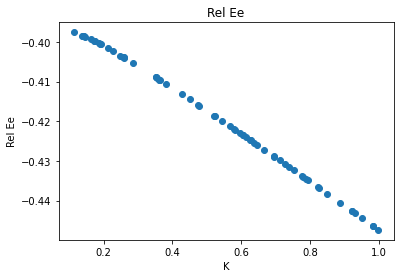
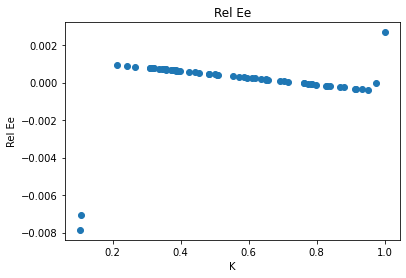
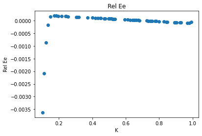
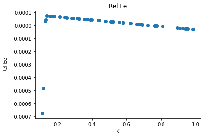
In order to be able to interpret the remaining errors in the equilibrium condition, we reformulate it such that deviations from 0 can be interpreted as relative consumption errors:

\begin{align*} 0 &= -\frac{1}{C_t} + \beta \frac{1}{C_{t+1}}\left(1 - \delta + r_{t+1}\right) \tag{16} \\ \Leftrightarrow \frac{1}{C_t} &= \beta \frac{1}{C_{t+1}}\left(1 - \delta + r_{t+1}\right) \tag{17} \\ \Leftrightarrow C_t &= \frac{C_{t+1}}{\beta \left(1 - \delta + r_{t+1}\right)} \tag{18} \\ \Leftrightarrow 1 &= \frac{C_{t+1}}{C_t \beta \left(1 - \delta + r_{t+1}\right)} \tag{19} \\ \Leftrightarrow 0 &= \frac{C_{t+1}}{C_t \beta \left(1 - \delta + r_{t+1}\right)} - 1. \tag{20} \end{align*}

We will encode this equation as the loss function to train the neural network.
I.e. we will train the neural network $\mathcal{N}(\cdot)$ such that the implied policy fullfills the equation above.
Two remarks are in order:

The above function can’t be evaluated correctly if consumption or the level of capital are not positive. Since a neural network is initialized randomly, this is not guaranteed by itself. One way to address both reqirements is to approximate the savings rate $s_t$ , such that $K_{t+1} = (1 - \delta) K_t + Y_t s_t =(1 - \delta) K_t + Y_t \mathcal{N}(K_t)$ . Since $Y_t$ is completely determined given the state $K_t$ , this formulation still encodes the policy $K_{t+1}$ , albeit slightly more indirectly. Using a sigmoid activation function we can ensure that $s_t\in(0, 1)$ and hence $K_{t+1}\geq 0$ and $C_t\geq 0$ . In settings where this is not possible, measure would have to be taken (such as replacing negative numbers by small positive numbers and then adding a punishment term to the loss function), which help the neural network in the beginning of training.
An important question is for what states we want the above equation to hold. In principle we want to hold it for all possible states $K_t$ , but in practice we need to focus on a finite space. In this notebook we startout in the simplest possible way and sample capital from an exogenous interval $\mathcal{K}=[\underline{K}, \overline{K}]$ , for which we know that $f(\mathcal{K})\in \mathcal{K}$ . When the state space is high dimensional, it is advantageous to sample more carefully, for example from the simulated path of the economy, i.e. from the ergodic distribution of states, that will be visited in equilibrium (see Maliar et al. (2011) for more information on this topic). The next notebook will show how this can be done using Deep Equilibrium Nets, here we will sample exogenously for simplicity.

Implementing the loss function¶

First, we need to import necessary python numerical libraries and tensorflow:

# Import necessary libraries
import numpy as np
import math
import tensorflow as tf
from tensorflow import keras

import matplotlib.pyplot as plt
from matplotlib import rc
plt.rcParams["font.size"] = 15

%matplotlib inline


# Reproducibility: fix seeds across numpy and TensorFlow (SEED from cell 2).
np.random.seed(SEED)
tf.random.set_seed(SEED)

print("Version of tensorflow is {}".format(tf.__version__))

2026-04-24 07:19:30.703589: E external/local_xla/xla/stream_executor/cuda/cuda_fft.cc:477] Unable to register cuFFT factory: Attempting to register factory for plugin cuFFT when one has already been registered
WARNING: All log messages before absl::InitializeLog() is called are written to STDERR
E0000 00:00:1777007970.729031   78937 cuda_dnn.cc:8310] Unable to register cuDNN factory: Attempting to register factory for plugin cuDNN when one has already been registered
E0000 00:00:1777007970.735583   78937 cuda_blas.cc:1418] Unable to register cuBLAS factory: Attempting to register factory for plugin cuBLAS when one has already been registered
2026-04-24 07:19:30.762127: I tensorflow/core/platform/cpu_feature_guard.cc:210] This TensorFlow binary is optimized to use available CPU instructions in performance-critical operations.
To enable the following instructions: AVX2 FMA, in other operations, rebuild TensorFlow with the appropriate compiler flags.

Version of tensorflow is 2.18.0

We define the economic parameters, which are constant throughout and will be globals in this notebook.

alpha = 0.36  # Capital share in the Cobb-Douglas production function
beta = 0.99  # Discount factor
delta = 1.0 # depreciation of capital

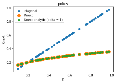
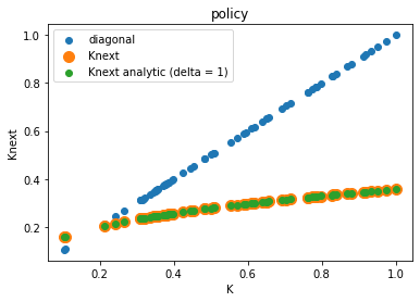
Since this model can be solved analytically for the full depreciation case, we implement the analytical solution (so that we can later check the solution found by the neural network).

def k_compute_infty(alpha, beta):
    """ Return the stationary point (or steady state) for full depreciation """
    return (1 / (beta * alpha))**(1/(alpha - 1))

k_infty = k_compute_infty(alpha, beta)
print("Stationary point is {:5f}".format(k_infty))


def Kplus_compute_analytic(K, alpha, beta):
    """ Return the optimal capital stock in the next period  for full depreciation """
    return alpha * beta * K**alpha


def c_compute(K, Knext, alpha, beta):
    """ Optimal consumption today given (K_t, K_{t+1}) for full depreciation: C_t = K_t^alpha - K_{t+1}. """
    return K**alpha - Knext

Stationary point is 0.199482

Deep neural network¶

In this section, we define the architecture of the deep neural net.
Our goal is for the neural network to approximate the savings rate $s_t$ , such that $K_{t+1} = Y_t s_t \approx Y_t \mathcal{N}\left(K_t \right)$ .
The neural network input is hence a 1-dimensional state $K_t$ and the output is the 1-dimensional savings rate $s_t$ .

Hyper parameters¶

Hyper parameter defines the architecture of the deep neural net.
Note that the purpose of this notebook is in the demonstration of the deep neural net. Detail analyses of the choice of hyper parameters are omitted and we use a densely connected feed forward neural network with two hidden layers as in Azinovic et al. (2022). Since we are approximating the savings rate, we want our architecture to ensure that $s_t \in (0, 1)$ . We can do this by using a sigmoid activation function in the output layer. This is in the spirit of encoding prior knowledge based on economics directly into the neural network architecture (relatedly, Kahou et al. (2021) and Han et al. (2022) show how symmetry can be encoded into the neural-network architecture and Azinovic and Žemlička (2023) introduce market clearing neural network architectures.). We assume the following structure of layers and activation functions:
- Layer 1: the input layer, 1 neuron corresponding to the capital stock $K_t$
- Layer 2: the first hidden layer, 50 neurons and is activated by Relu
- Layer 3: the second hidden layer, 50 neurons and is activated by Relu
- Layer 4: the output layer, 1 neuron corresponding to the savings rate $s_t$ , such that $K_{t+1}=(1 - \delta) K_t + Y_t s_t$ . We use a sigmoid activation function, ensuring that $s_t \in (0, 1)$ .

# Layer setting
num_input = 1
num_hidden1 = 50
num_hidden2 = 50
num_output = 1
layers_dim = [num_input, num_hidden1, num_hidden2, num_output]
print("Dimensions of each layer are {}".format(layers_dim))

Dimensions of each layer are [1, 50, 50, 1]

We define the neural network¶

We use Keras to define the neural network

Hard vs. soft constraints — the central design choice in DEQNs¶

Two kinds of equilibrium conditions appear in any dynamic stochastic model:

Inequality / feasibility constraints — e.g.\ $C_t > 0$ , $K_{t+1} > 0$ , the resource constraint $C_t + K_{t+1} = Y_t$ . These must hold exactly.
Optimality conditions — e.g.\ the Euler equation. These hold in the equilibrium but not at every intermediate guess of the policy.

Azinovic, Gaegauf & Scheidegger (2022, §4.2.2; lecture script Fig. 2.3) make this distinction explicit and treat the two kinds very differently:

	Hard constraint (architecture)	Soft constraint (loss)
What	Built into the network output	Penalised in the cost function
How	Activation choice + algebraic identities	Squared residuals in $\mathcal{L}$
Cost	Always satisfied — even at random init	Only satisfied at convergence

Why this matters here. The cell below parameterises the savings share $s_t \in (0, 1)$ via a sigmoid output. Combined with the resource constraint $K_{t+1} = s_t Y_t$ and $C_t = (1 - s_t) Y_t$ , this guarantees $C_t > 0$ and $K_{t+1} > 0$ simultaneously, at every iteration of training. We never have to penalise infeasibility — the architecture rules it out. The Euler equation, by contrast, is enforced softly through the loss.

This split removes a whole class of bad local minima (network outputs that would imply $C_t < 0$ ) and is one reason DEQNs converge in regions where naive penalty methods do not.

# we use sigmod in the output layer so output is between 0 and 1
nn = keras.Sequential([
    keras.layers.Dense(num_hidden1, activation='relu', input_shape=(num_input,)),
    keras.layers.Dense(num_hidden2, activation='relu'),
    keras.layers.Dense(num_output, activation='sigmoid')
])

/usr/local/lib/python3.10/dist-packages/keras/src/layers/core/dense.py:87: UserWarning: Do not pass an `input_shape`/`input_dim` argument to a layer. When using Sequential models, prefer using an `Input(shape)` object as the first layer in the model instead.
  super().__init__(activity_regularizer=activity_regularizer, **kwargs)
2026-04-24 07:19:35.204986: E external/local_xla/xla/stream_executor/cuda/cuda_driver.cc:152] failed call to cuInit: INTERNAL: CUDA error: Failed call to cuInit: UNKNOWN ERROR (303)

print(nn.summary())

None

The batch dimension¶

Since neural networks are highly parallelizable, we typically do not want to evaluate the neural network for only a single state $K \in \mathbb{R}$ , but for a vector of $N_{data}$ different capital levels $\mathbf{K} \in \mathbb{R}^{N_{data}\times 1}$ . The output of the neural network is then a vector $\mathbf{s}\in \mathbb{R}^{N_{data}\times 1}$ .
The convention in deep learning is to have the different data samples on the 0-axis.

# test it
K_test = np.array([[1.], [2.]])

print("K_test = ", K_test)
print("nn prediction = ", nn(K_test))

K_test =  [[1.]
 [2.]]
nn prediction =  tf.Tensor(
[[0.518157  ]
 [0.53626615]], shape=(2, 1), dtype=float32)

Implementing the cost function¶

As outlined above, we want to implement a cost-function which takes a vector of states $\mathbb{X}\in \mathbb{R}^{N_{data}\times 1}$ and a neural network $\mathcal{N}(\cdot)$ , and then returns a vector of errors in the equilibrium conditions implied by the policy, which is encoded by the neural network.
As explained above, the equilibrium condition is given by

\begin{align} 0 &= \frac{C_{t+1}}{C_t \beta \left(1 - \delta + r_{t+1}\right)} - 1. \end{align}

(21)

We use the tf.function decorator, which speeds up the evaluation of the cost function.

@tf.function
def compute_cost(X, nn):
    """ 
    Compute the mean squared error in the equilibrium conditions.
    """
    n_data = X.shape[0] # number of states is on the axis 0
    dim_state = X.shape[1] # dimensionality of the state is on axis 1
    
    # read out the state (this is trivial here because the state-space is one dimensional)
    K_t = X
    
    # compute output today
    Y_t = K_t ** alpha
    
    # use the neural network to predict the savings rate
    s_t = nn(X)
    
    # get the implied capital in the next period
    K_tplus1 = (1. - delta) * K_t + Y_t * s_t

    C_t = Y_t - Y_t * s_t
    
    # get the state in t + 1
    X_next = K_tplus1
     
    # get output in the next period
    Y_tplus1 = K_tplus1 ** alpha
    
    # predict the savings policy in the next period
    s_tplus1 = nn(X_next)
    
    # predict capital in the next period
    C_tplus1 = Y_tplus1 - s_tplus1 * Y_tplus1
    
    # compute the return on capital in the next period
    R_tplus1 = alpha * K_tplus1 ** (alpha - 1.)
    
    # Define the relative Euler error
    errREE = 1 - C_tplus1 / (beta * C_t * (R_tplus1 + 1. - delta))
    
    # compute the cost, i.e. the mean square error in the equilibrium conditions
    cost = tf.reduce_mean(errREE ** 2)

    return cost, errREE, C_t, C_tplus1, K_tplus1, R_tplus1

# let's try
X = tf.constant([[1.], [2.], [3.]])

print("cost = ", compute_cost(X, nn)[0])

cost =  tf.Tensor(0.34953928, shape=(), dtype=float32)

Gradients¶

Now we define a function that, for given data X, computes the gradient of the loss w.r.t. the neural network parameters.
This gradient will be used to update the neural network parameters into the direction which decreases the loss function.

def grad(X, nn):
    with tf.GradientTape() as tape:
        loss_value = compute_cost(X, nn)[0]
    return loss_value, tape.gradient(loss_value, nn.trainable_variables)

X = tf.constant([[1.], [2.], [3.]])

loss, grads = grad(X, nn)

print("loss = ", loss)
print("grads = ", grads)

loss =  tf.Tensor(0.34953928, shape=(), dtype=float32)
grads =  [<tf.Tensor: shape=(1, 50), dtype=float32, numpy=
array([[ 0.        ,  0.        , -0.08185728,  0.        ,  0.        ,
         0.7403764 ,  0.        ,  0.        , -0.02748141, -0.18520665,
         0.        ,  0.93225586,  0.39725724,  0.6557343 ,  0.        ,
         0.        ,  0.        ,  0.06075807, -0.48891822,  0.35522285,
         0.        , -0.22779387,  0.        ,  0.12700742,  0.45544162,
        -0.17668146, -0.9804636 , -0.34549388,  0.20925799,  0.        ,
        -0.32901508,  0.2908884 ,  0.        ,  0.18590003,  0.        ,
         0.        ,  0.        , -0.8201485 ,  0.        , -0.12001515,
         0.486988  ,  0.        ,  0.        ,  0.        , -0.3768868 ,
         0.        ,  0.        , -0.40578467, -0.71164227, -0.30819616]],
      dtype=float32)>, <tf.Tensor: shape=(50,), dtype=float32, numpy=
array([ 0.        ,  0.        , -0.02189168,  0.        ,  0.        ,
        0.19800422,  0.        ,  0.        , -0.00734955, -0.04953115,
        0.        ,  0.24931997,  0.10624138,  0.17536777,  0.        ,
        0.        ,  0.        ,  0.01624897, -0.13075495,  0.09499982,
        0.        , -0.06092056,  0.        ,  0.03396651,  0.12180206,
       -0.0472512 , -0.26221246, -0.09239791,  0.05596337,  0.        ,
       -0.08799087,  0.0777944 ,  0.        ,  0.04971658,  0.        ,
        0.        ,  0.        , -0.21933827,  0.        , -0.03209652,
        0.13023871,  0.        ,  0.        ,  0.        , -0.10079357,
        0.        ,  0.        , -0.10852191, -0.1903196 , -0.08242313],
      dtype=float32)>, <tf.Tensor: shape=(50, 50), dtype=float32, numpy=
array([[0.        , 0.        , 0.        , ..., 0.        , 0.        ,
        0.        ],
       [0.        , 0.        , 0.        , ..., 0.        , 0.        ,
        0.        ],
       [0.20554706, 0.        , 0.        , ..., 0.        , 0.        ,
        0.        ],
       ...,
       [0.20257655, 0.        , 0.        , ..., 0.        , 0.        ,
        0.        ],
       [0.09174025, 0.        , 0.        , ..., 0.        , 0.        ,
        0.        ],
       [0.03313174, 0.        , 0.        , ..., 0.        , 0.        ,
        0.        ]], dtype=float32)>, <tf.Tensor: shape=(50,), dtype=float32, numpy=
array([ 0.25610134,  0.        ,  0.        ,  0.        ,  0.06923579,
        0.13579926,  0.2714291 ,  0.        ,  0.        ,  0.        ,
        0.20293039,  0.27493438,  0.        ,  0.        ,  0.21134631,
        0.        ,  0.05500378,  0.        , -0.0485963 ,  0.        ,
        0.06831585,  0.        ,  0.00114351,  0.        ,  0.        ,
       -0.25841826,  0.01841421, -0.10364143,  0.05056649,  0.        ,
       -0.24315876,  0.25273582,  0.23932949,  0.24390697, -0.27987036,
        0.        ,  0.        ,  0.        ,  0.04946745,  0.        ,
       -0.18767306,  0.        ,  0.        ,  0.        ,  0.18389553,
       -0.19852278,  0.        ,  0.        ,  0.        ,  0.        ],
      dtype=float32)>, <tf.Tensor: shape=(50, 1), dtype=float32, numpy=
array([[3.2589558e-01],
       [0.0000000e+00],
       [0.0000000e+00],
       [0.0000000e+00],
       [6.8967298e-02],
       [4.4044530e-01],
       [6.2575683e-02],
       [0.0000000e+00],
       [0.0000000e+00],
       [0.0000000e+00],
       [2.4744456e-01],
       [1.9941750e-01],
       [0.0000000e+00],
       [0.0000000e+00],
       [9.8374540e-01],
       [0.0000000e+00],
       [6.4311647e-01],
       [0.0000000e+00],
       [1.7349435e-01],
       [0.0000000e+00],
       [3.5381091e-01],
       [0.0000000e+00],
       [3.2913262e-01],
       [0.0000000e+00],
       [0.0000000e+00],
       [3.8304621e-01],
       [1.3592526e-01],
       [3.1626534e-01],
       [7.1445544e-04],
       [0.0000000e+00],
       [3.1197363e-01],
       [1.0957710e-01],
       [3.7392193e-01],
       [5.3837115e-01],
       [8.4311974e-01],
       [0.0000000e+00],
       [0.0000000e+00],
       [0.0000000e+00],
       [1.8321347e-01],
       [0.0000000e+00],
       [7.9091579e-01],
       [0.0000000e+00],
       [0.0000000e+00],
       [0.0000000e+00],
       [1.8371603e-01],
       [8.5727826e-02],
       [0.0000000e+00],
       [0.0000000e+00],
       [0.0000000e+00],
       [0.0000000e+00]], dtype=float32)>, <tf.Tensor: shape=(1,), dtype=float32, numpy=array([0.8881669], dtype=float32)>]

Optimizer¶

We now define an optimizer, essentially an improved version of SGD

learning_rate = 0.001
optimizer = tf.keras.optimizers.Adam(learning_rate=learning_rate)

Sampling data¶

we make a function to generate training data. Here we just sample exogenously from an interval.

def get_training_data(k_lb, k_ub, n_data):
    X = tf.random.uniform(
    shape = [n_data, 1],
    minval=k_lb,
    maxval=k_ub,
    dtype=tf.dtypes.float32)
    return X

Training¶

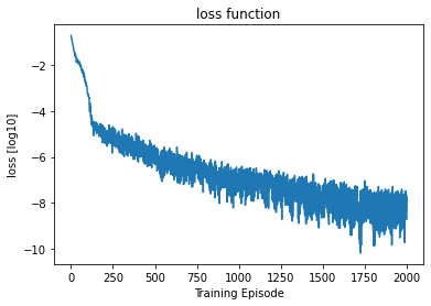
We iteratively generate training data and update the neural network

# Keep results for plotting
train_loss = []

num_episodes = NUM_EPISODES
n_data_per_epi = 64
k_lb = 0.10
k_ub = 1.0


for ep in range(num_episodes):
    # generate training data
    X = get_training_data(k_lb, k_ub, n_data_per_epi)

    # compute loss and gradients
    loss, grads = grad(X, nn)
    
    # apply gradients
    optimizer.apply_gradients(zip(grads, nn.trainable_variables))
    
    # record loss
    train_loss.append(loss.numpy())
    
    # print progress
    if ep % 100 == 0:
        print("#=================================================================")
        print("episode = {}, loss [log10] = {}".format(ep, np.log10(loss.numpy())))
        
    if ep % 500 == 0:
        cost, errREE, C_t, C_tplus1, K_tplus1, R_tplus1 = compute_cost(X, nn)
        
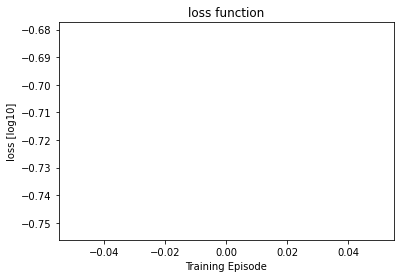
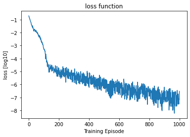
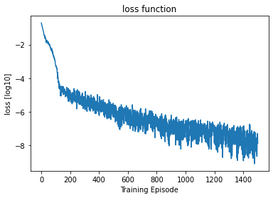
        plt.title("loss function")
        plt.plot(np.log10(np.array(train_loss)))
        plt.xlabel("Training Episode")
        plt.ylabel("loss [log10]")
        plt.show()
        plt.close()

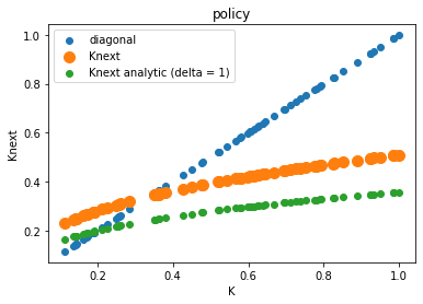
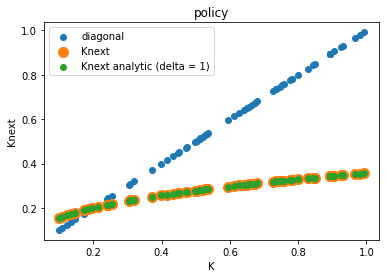
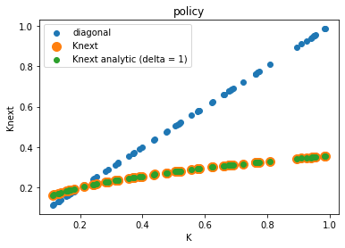
        plt.title("policy")
        plt.xlabel("K")
        plt.ylabel("Knext")
        plt.scatter(X[:, 0], X[:, 0], label = "diagonal")
        plt.scatter(X[:, 0], K_tplus1[:, 0], s=100, label = "Knext")
        plt.scatter(X[:, 0], beta * alpha * X[:, 0] ** alpha, label = "Knext analytic (delta = 1)")
        plt.legend()
        plt.show()
        plt.close()

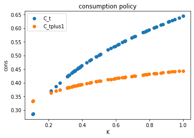
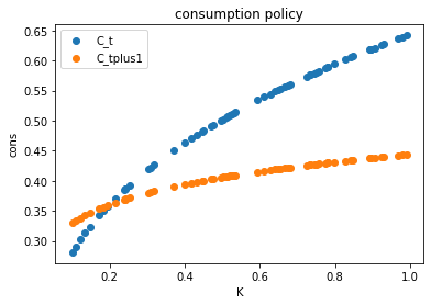
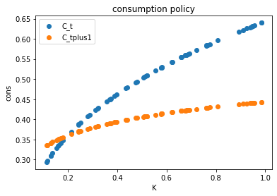
        plt.title("consumption policy")
        plt.xlabel("K")
        plt.ylabel("cons")
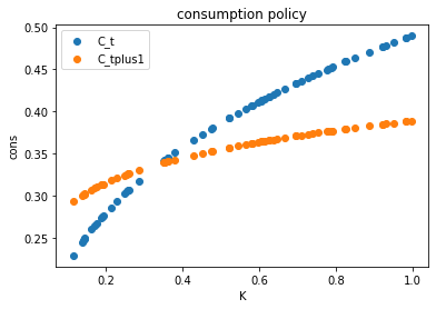
        plt.scatter(X[:, 0], C_t[:, 0], label="C_t")
        plt.scatter(X[:, 0], C_tplus1[:, 0], label="C_tplus1")
        plt.legend()
        plt.show()
        plt.close()

        plt.title("Rel Ee")
        plt.xlabel("K")
        plt.ylabel("Rel Ee")
        plt.scatter(X[:, 0], errREE[:, 0], label="REE")
        plt.show()
        plt.close()
       
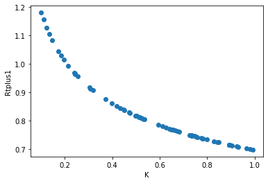
        plt.xlabel("K")
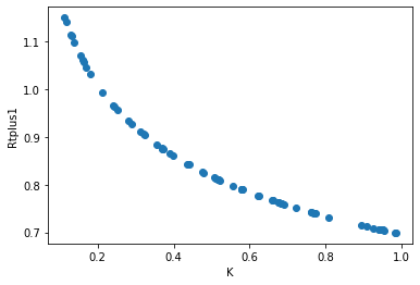
        plt.ylabel("Rtplus1")
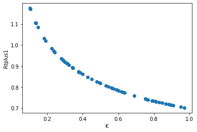
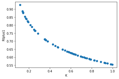
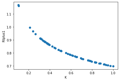
        plt.scatter(X[:, 0], R_tplus1[:, 0], label="R_tplus1")
        plt.show()
        plt.close()

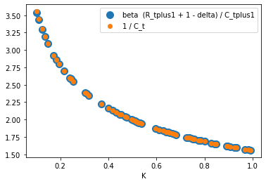
        plt.xlabel("K")
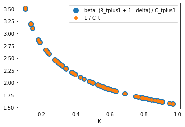
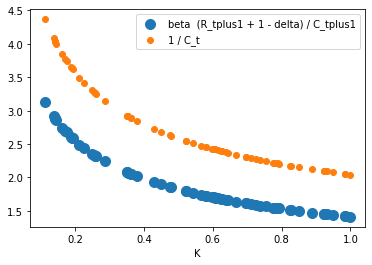
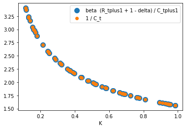
        plt.scatter(X[:, 0], beta * (R_tplus1[:, 0] + 1. - delta)/C_tplus1[:, 0], s=100, label="beta  (R_tplus1 + 1 - delta) / C_tplus1")
        plt.scatter(X[:, 0], 1/C_t[:, 0], label="1 / C_t")
        plt.legend()
        plt.show()
        plt.close()

#=================================================================
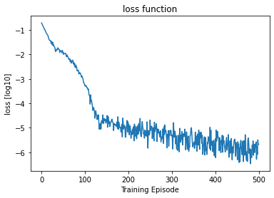
episode = 0, loss [log10] = -0.7167789936065674

#=================================================================
episode = 100, loss [log10] = -3.2881734371185303

#=================================================================
episode = 200, loss [log10] = -4.882792949676514

#=================================================================
episode = 300, loss [log10] = -5.282750606536865

#=================================================================
episode = 400, loss [log10] = -5.449318885803223

#=================================================================
episode = 500, loss [log10] = -5.677831172943115

#=================================================================
episode = 600, loss [log10] = -5.915491104125977

#=================================================================
episode = 700, loss [log10] = -6.517192840576172

#=================================================================
episode = 800, loss [log10] = -6.443454742431641

#=================================================================
episode = 900, loss [log10] = -6.203360080718994

#=================================================================
episode = 1000, loss [log10] = -6.529022216796875

#=================================================================
episode = 1100, loss [log10] = -7.242496967315674

#=================================================================
episode = 1200, loss [log10] = -6.812475204467773

#=================================================================
episode = 1300, loss [log10] = -7.430716514587402

#=================================================================
episode = 1400, loss [log10] = -8.797263145446777

#=================================================================
episode = 1500, loss [log10] = -7.885437965393066

#=================================================================
episode = 1600, loss [log10] = -7.846672534942627

#=================================================================
episode = 1700, loss [log10] = -8.730031967163086

#=================================================================
episode = 1800, loss [log10] = -7.586095333099365

#=================================================================
episode = 1900, loss [log10] = -7.722903728485107

#=================================================================
episode = 2000, loss [log10] = -7.661026954650879