Course: Deep Learning for Solving and Estimating Dynamic Models in Economics and Finance
Script reference: §1.5–1.8 (Optimization and training: PyTorch fundamentals)
Notebook role: core
Author: Simon Scheidegger
RUN_MODE = "smoke"  # one of: "smoke", "teaching", "production"
SEED = 0
Introduction to Deep Learning with PyTorch: Neural Networks for Regression and Classification¶
In this notebook, we demonstrate how to build neural network models for both regression and classification tasks using PyTorch. Only neural networks (i.e., multi-layer perceptrons) are used.
The notebook is organized as follows:
Regression Example:
Generate synthetic regression data.
Build a neural network with a hidden layer to learn the relationship.
Train the network using Mean Squared Error (MSE) loss and visualize the results.
Classification Example:
Generate synthetic data for binary classification.
Build a neural network with a hidden layer for classification.
Train the network using Binary Cross-Entropy (BCE) loss and visualize the decision boundary.
Let’s begin by setting up our environment.
import torch
import torch.nn as nn
import torch.optim as optim
import numpy as np
import matplotlib.pyplot as plt

%matplotlib inline

# Set random seeds for reproducibility
torch.manual_seed(SEED)
np.random.seed(SEED)
1. Regression Example with a Neural Network¶
We generate synthetic regression data following the relationship:
We then build a neural network with one hidden layer to learn this relationship.
# Generate synthetic regression data
n_samples = 100
X_reg = np.linspace(0, 1, n_samples)
y_reg = 2 * X_reg + 1 + np.random.normal(0, 0.1, n_samples)

# Convert the data to torch tensors (shape: [n_samples, 1])
X_reg_tensor = torch.tensor(X_reg, dtype=torch.float32).unsqueeze(1)
y_reg_tensor = torch.tensor(y_reg, dtype=torch.float32).unsqueeze(1)

# Plot the synthetic data
plt.figure(figsize=(8, 5))
plt.scatter(X_reg, y_reg, color="blue", label="True Data")
plt.xlabel("X")
plt.ylabel("y")
plt.title("Synthetic Regression Data")
plt.legend()
plt.show()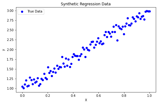
Neural Network Model for Regression¶
We define a simple neural network with:
An input layer of dimension 1.
One hidden layer with 10 neurons and ReLU activation.
An output layer of dimension 1 (for regression output).
class RegressionNN(nn.Module):
    def __init__(self, input_dim=1, hidden_dim=1000, output_dim=1):
        super(RegressionNN, self).__init__()
        self.net = nn.Sequential(
            nn.Linear(input_dim, hidden_dim),
            nn.ReLU(),
            nn.Linear(hidden_dim, output_dim)
        )

    def forward(self, x):
        return self.net(x)

# Initialize the regression neural network
model_reg = RegressionNN()
Training the Regression Model¶
We use the Mean Squared Error (MSE) loss function and the Adam optimizer.
criterion_reg = nn.MSELoss()
optimizer_reg = optim.Adam(model_reg.parameters(), lr=0.01)

n_epochs = 1000
loss_history_reg = []

for epoch in range(n_epochs):
    optimizer_reg.zero_grad()             # Zero the gradients
    outputs = model_reg(X_reg_tensor)       # Forward pass
    loss = criterion_reg(outputs, y_reg_tensor)  # Compute loss
    loss.backward()                       # Backward pass
    optimizer_reg.step()                  # Update parameters
    loss_history_reg.append(loss.item())

    if (epoch + 1) % 200 == 0:
        print(f"Epoch {epoch+1}/{n_epochs}, Loss: {loss.item():.4f}")
Epoch 200/1000, Loss: 0.0076
Epoch 400/1000, Loss: 0.0074
Epoch 600/1000, Loss: 0.0073
Epoch 800/1000, Loss: 0.0072
Epoch 1000/1000, Loss: 0.0071
# Plot training loss
plt.figure(figsize=(8, 5))
plt.plot(loss_history_reg)
plt.xlabel("Epoch")
plt.ylabel("MSE Loss")
plt.title("Regression Training Loss")
plt.show()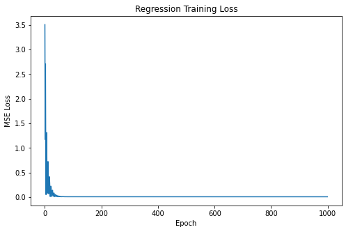
Visualizing the Regression Results¶
We compare the neural network predictions to the true data.
with torch.no_grad():
    predictions = model_reg(X_reg_tensor).numpy()

plt.figure(figsize=(8, 5))
plt.scatter(X_reg, y_reg, color="blue", label="True Data")
plt.plot(X_reg, predictions, color="red", label="NN Predictions")
plt.xlabel("X")
plt.ylabel("y")
plt.title("Regression: True Data vs. NN Predictions")
plt.legend()
plt.show()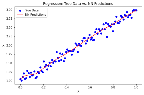
2. Classification Example with a Neural Network¶
Next, we create a binary classification task by generating synthetic data from two distinct Gaussian distributions. We then build a neural network with one hidden layer to classify the data.
# Generate synthetic classification data
n_samples_class = 100

# Class 0: centered at (-2, -2)
X_class0 = np.random.randn(n_samples_class, 2) + np.array([-2, -2])
y_class0 = np.zeros(n_samples_class)

# Class 1: centered at (2, 2)
X_class1 = np.random.randn(n_samples_class, 2) + np.array([2, 2])
y_class1 = np.ones(n_samples_class)

# Combine the data for both classes
X_class = np.vstack((X_class0, X_class1))
y_class = np.hstack((y_class0, y_class1))

# Convert data to torch tensors
X_class_tensor = torch.tensor(X_class, dtype=torch.float32)
y_class_tensor = torch.tensor(y_class, dtype=torch.float32).unsqueeze(1)

# Plot the synthetic classification data
plt.figure(figsize=(8, 5))
plt.scatter(X_class[:, 0], X_class[:, 1], c=y_class, cmap="bwr", edgecolors="k", alpha=0.7)
plt.xlabel("Feature 1")
plt.ylabel("Feature 2")
plt.title("Synthetic Classification Data")
plt.show()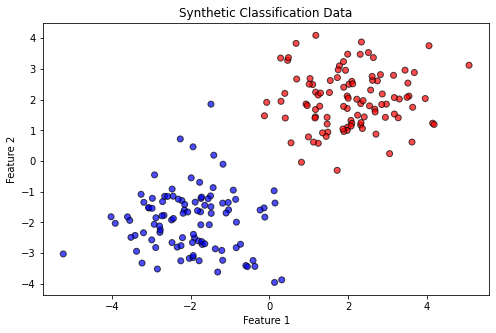
Neural Network Model for Classification¶
We define a neural network with:
An input layer of dimension 2.
One hidden layer with 10 neurons and ReLU activation.
An output layer with 1 neuron followed by a Sigmoid activation (to output probabilities).
class ClassificationNN(nn.Module):
    def __init__(self, input_dim=2, hidden_dim=10, output_dim=1):
        super(ClassificationNN, self).__init__()
        self.net = nn.Sequential(
            nn.Linear(input_dim, hidden_dim),
            nn.ReLU(),
            nn.Linear(hidden_dim, output_dim),
            nn.Sigmoid()  # Sigmoid activation for probability output
        )

    def forward(self, x):
        return self.net(x)

# Initialize the classification neural network
model_class = ClassificationNN()
Training the Classification Model¶
We use the Binary Cross-Entropy (BCE) loss function and the Adam optimizer for training.
criterion_class = nn.BCELoss()
optimizer_class = optim.Adam(model_class.parameters(), lr=0.01)

n_epochs_class = 1000
loss_history_class = []

for epoch in range(n_epochs_class):
    optimizer_class.zero_grad()               # Zero the gradients
    outputs = model_class(X_class_tensor)       # Forward pass
    loss = criterion_class(outputs, y_class_tensor)  # Compute BCE loss
    loss.backward()                           # Backward pass
    optimizer_class.step()                      # Update parameters
    loss_history_class.append(loss.item())

    if (epoch + 1) % 200 == 0:
        print(f"Epoch {epoch+1}/{n_epochs_class}, Loss: {loss.item():.4f}")
Epoch 200/1000, Loss: 0.0047
Epoch 400/1000, Loss: 0.0017
Epoch 600/1000, Loss: 0.0009
Epoch 800/1000, Loss: 0.0005
Epoch 1000/1000, Loss: 0.0004
# Plot classification training loss
plt.figure(figsize=(8, 5))
plt.plot(loss_history_class)
plt.xlabel("Epoch")
plt.ylabel("BCE Loss")
plt.title("Classification Training Loss")
plt.show()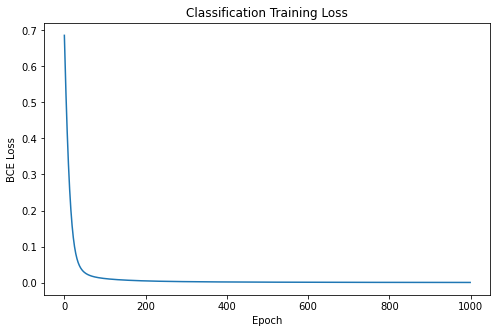
Visualizing the Decision Boundary¶
We generate a grid of points across the feature space, predict their class probabilities, and then plot the decision boundary.
# Create a grid over the feature space
x_min, x_max = X_class[:, 0].min() - 1, X_class[:, 0].max() + 1
y_min, y_max = X_class[:, 1].min() - 1, X_class[:, 1].max() + 1
xx, yy = np.meshgrid(np.linspace(x_min, x_max, 200),
                     np.linspace(y_min, y_max, 200))
grid = np.c_[xx.ravel(), yy.ravel()]
grid_tensor = torch.tensor(grid, dtype=torch.float32)

# Compute model predictions on the grid
with torch.no_grad():
    preds_grid = model_class(grid_tensor).reshape(xx.shape).numpy()

# Plot the decision boundary and the data
plt.figure(figsize=(8, 5))
plt.contourf(xx, yy, preds_grid, levels=[0, 0.5, 1], alpha=0.3, colors=["blue", "red"])
plt.scatter(X_class[:, 0], X_class[:, 1], c=y_class, cmap="bwr", edgecolors="k", alpha=0.7)
plt.xlabel("Feature 1")
plt.ylabel("Feature 2")
plt.title("Classification: Decision Boundary")
plt.show()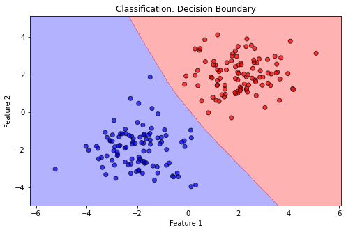
Conclusion¶
In this notebook, we introduced deep learning with PyTorch using neural networks exclusively for both regression and classification tasks.
For regression, we built a neural network with one hidden layer to learn a simple linear relationship with noise.
For classification, we constructed a neural network with one hidden layer to distinguish between two classes generated from distinct Gaussian distributions.
These examples serve as a foundation for exploring more complex neural network architectures and deep learning techniques with PyTorch.