Lecture 02, Notebook 02: Gradient Descent and Stochastic Gradient Descent

Course: Deep Learning for Solving and Estimating Dynamic Models in Economics and Finance
Script reference: §1.5 (Optimization: gradient descent, SGD, mini-batch, learning rate)
Notebook role: core
Author: Simon Scheidegger

Gradient and Stochastic Gradient Descent¶

This notebook is adjusted from https://nbviewer.jupyter.org/github/dtnewman/gradient_descent/blob/master/stochastic_gradient_descent.ipynb

Gradient Descent¶

• Gradient descent, also known as steepest descent, is an optimization algorithm for finding the local minimum of a function.

• To find a local minimum, the function “steps” in the direction of the negative of the gradient.

• Gradient ascent is the same as gradient descent, except that it steps in the direction of the positive of the gradient and therefore finds local maxima instead of minima. The algorithm of gradient descent can be outlined as follows:

    1:   Choose initial guess $x_0$
    2:   for k = 0, 1, 2, ... do
    3:       $s_k$ = -$\nabla f(x_k)$
    4:       choose $\alpha_k$ to minimize $f(x_k+\alpha_k s_k)$
    5:       $x_{k+1} = x_k + \alpha_k s_k$
    6:   end for

As an analytical example, we try to find a local minimum for the function $f(x) = x^3-2x^2+2$

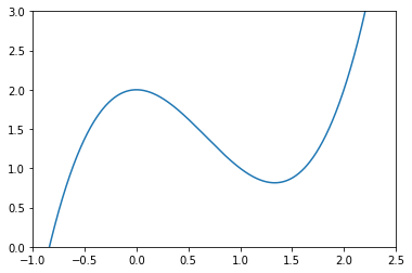
We can see from the graph above that our local minimum is gonna be around 1.4 (on the x-axis).

Let’s pretend that we don’t know that, so we set our starting point (arbitrarily, in this case) at $x_0 = 2$

The figures below show step-by-step the route that was taken to find the local minimum.

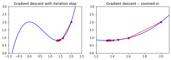
Note: that the step size (also called learning rate) in the implementation above is constant.

->Doing this makes it easier to implement the algorithm. 

However, it also presents some issues:

• If the step size is too small, then convergence might be very slow.

• If we make it too large, then the method may fail to converge at all.

  -> A solution to this is to use adaptive step sizes as the algorithm below does (using scipy’s fmin function to find optimal step sizes)

• With adaptive step sizes, the algorithm converges in just 4 iterations rather than 17.

• Note: it also takes extra time to compute the appropriate step size at each iteration.

Below are some plots of the path taken below.

You can see that it converges very quickly to a point near the local minimum, so it’s hard to even discern the dots after the first two steps until we zoom in very close in the third frame below.

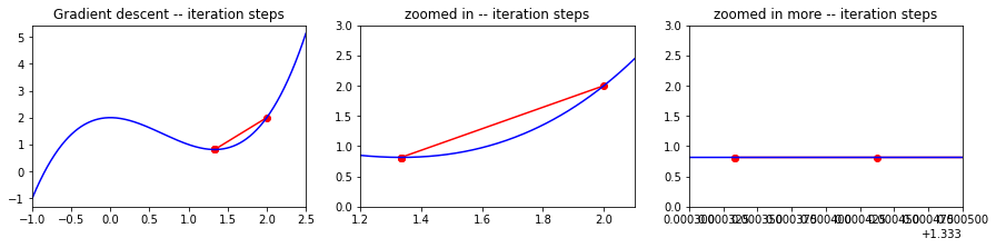
An alternative approach to update the step size is to choose a decrease constant $d$ that shrinks the step size over time: $\eta(t+1) = \eta(t) / (1+t \times d)$.

A more complicated example¶

• Consider a simple linear regression where we want to see how the temperature affects the noises made by crickets.

• There is a data set of cricket chirp rates at various temperatures.

• First we’ll load that data set in and plot it:

Data: cricket chirp rate vs temperature¶

SGD_data.txt is a 16-row, two-column CSV with no header. Column 1: chirps per second (striped ground cricket, Gryllus rubens).
Column 2: ambient temperature in degrees Fahrenheit.

This is a standard introductory dataset (originally from G. W. Pierce, The Songs of Insects, Harvard University Press, 1948) widely used to illustrate simple linear regression. It is included here as a minimal worked example for gradient descent: fitting $heta_0 + heta_1 x$ to the chirp-temperature relationship.

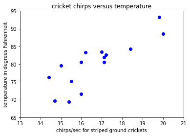
• Our goal is to find the parameters of a linear regression model---that is, the equation of the straight line

  $h_\theta(x) = \theta_0 + \theta_1 x$

  that best fits our data points.

• Thus, the function that we are trying to minimize in this case is:

  $J(\theta_0,\theta_1) = {1 \over m} \sum\limits_{i=1}^m (h_\theta(x_i)-y_i)^2$

• In this case, our gradient will be defined in two dimensions:

  $\frac{\partial}{\partial \theta_0} J(\theta_0,\theta_1) = \frac{1}{m} \sum\limits_{i=1}^m (h_\theta(x_i)-y_i)$

  $\frac{\partial}{\partial \theta_1} J(\theta_0,\theta_1) = \frac{1}{m} \sum\limits_{i=1}^m ((h_\theta(x_i)-y_i) \cdot x_i)$

Below, we set up our function for h, J and the gradient:

Now, we load our training data into the x and y variables:

Now, we run the gradient descent algorithm (without adaptive step sizes in this example):

For comparison, let’s get the actual values for $\theta_0$ and $\theta_1$:

• We can see that the values are relatively close to the actual values (even though our method was pretty slow). If you look at the source code of linregress, it uses the convariance matrix of x and y to compute fastly. Below, you can see a plot of the line drawn with our theta values against the data:

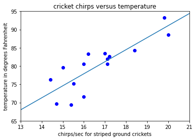
Notice that in the method above we need to calculate the gradient in every step of our algorithm.

• In the example with the crickets, this is not a big deal since there are only 15 data points.

• But imagine that we had 1 million data points.

• If this were the case, it would certainly make the method above far less efficient.

• In machine learning, the algorithm above is often called batch gradient descent to contrast it withmini-batch gradient descent (which we will not go into here) and stochastic gradient descent.

Stochastic gradient descent¶

• In batch gradient descent, we must look at every example in the entire training set on every step (in cases where a training set is used for gradient descent).

• This can be quite slow if the training set is sufficiently large.

• In stochastic gradient descent, we update our values after looking at each item in the training set, so that we can start making progress right away.

• Recall the linear regression example above. In that example, we calculated the gradient for each of the two theta values as follows:

  $\frac{\partial}{\partial \theta_0} J(\theta_0,\theta_1) = \frac{1}{m} \sum\limits_{i=1}^m (h_\theta(x_i)-y_i)$

  $\frac{\partial}{\partial \theta_1} J(\theta_0,\theta_1) = \frac{1}{m} \sum\limits_{i=1}^m ((h_\theta(x_i)-y_i) \cdot x_i)$

  Where $h_\theta(x) = \theta_0 + \theta_1 x$ and the per-example cost is $\tfrac{1}{2}(h_\theta(x_i)-y_i)^2$ (the $\tfrac{1}{2}$ absorbs the chain-rule factor of 2, which is why no 2 appears in the gradient or in the SGD update below).

• Then we followed this algorithm (where $\alpha$ was a non-adapting stepsize):

    1:   Choose initial guess $x_0$
    2:   for k = 0, 1, 2, ... do
    3:       $s_k$ = -$\nabla f(x_k)$
    4:       $x_{k+1} = x_k + \alpha s_k$
    5:   end for

• When the sample data had 15 data points as in the example above, calculating the gradient was not very costly.

• But for very large data sets, this would not be the case. So instead, we consider a stochastic gradient descent algorithm for simple linear regression such as the following, where m is the size of the data set:

    1:   Randomly shuffle the data set
    2:   for k = 0, 1, 2, ... do
    3:       for i = 1 to m do
    4:            $\begin{bmatrix} \theta_{0} \\ \theta_1 \\ \end{bmatrix}=\begin{bmatrix} \theta_0 \\ \theta_1 \\ \end{bmatrix}-\alpha\begin{bmatrix} (h_\theta(x_i)-y_i) \\ x_i(h_\theta(x_i)-y_i) \\ \end{bmatrix}$
    5:       end for
    6:   end for

• Typically, with stochastic gradient descent, you will run through the entire data set 1 to 10 times (see value for k in line 2 of the pseudocode above), depending on how fast the data is converging and how large the data set is.

• With batch gradient descent, we must go through the entire data set before we make any progress. With this algorithm though, we can make progress right away and continue to make progress as we go through the data set. Therefore, stochastic gradient descent is often preferred when dealing with large data sets.

• Unlike gradient descent, stochastic gradient descent will tend to oscillate near a minimum value rather than continuously getting closer. It may never actually converge to the minimum though.

• One way around this is to slowly decrease the step size $\alpha$ as the algorithm runs. However, this is less common than using a fixed $\alpha$.

An analytical example¶

Here we demonstrate the use of stochastic gradient descent for linear regression. In the example below, we’ll create a set of 500,000 points around the line $y = 4x+10+\epsilon$, for values of x between 0 and 100:

• We first randomly shuffle around our dataset.

• Note: in this example, this step isn’t strictly necessary since the data is already in a random order.

• However, that obviously may not always be the case:

• Now we setup our h function and our cost function, which we will use to check how the value is improving.

• Next, we run our stochastic gradient descent algorithm. To see it’s progress, we’ll take a cost measurement at every step.

• Every 10,000 steps, we’ll get an average cost from the last 10,000 steps and then append that to our cost_list variable.

• We will run through the entire list 10 times here:

As one can see, the values for $\theta_0$ and $\theta_1$ are close to their true values of 10 and 4.

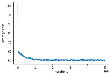
Next, we plot our cost versus the number of iterations. As you can see, the cost goes down quickly at first, but starts to level off as we go through more iterations: