Lecture 07, Notebook 02: Brock–Mirman via Autodiff (Deterministic)

Course: Deep Learning for Solving and Estimating Dynamic Models in Economics and Finance
Script reference: §2.7.3 (the autodiff Euler residual; Listing for the deterministic Brock–Mirman case)
Notebook role: core
Author: Simon Scheidegger

RUN_MODE = "smoke"  # one of: "smoke", "teaching", "production"
SEED = 0

# Chapter-wide RUN_MODE budget helper -- maps RUN_MODE to a training budget.
_BUDGET = {
    "smoke":      201,    # ~10 s, sanity check only
    "teaching":  2001,    # ~1 min CPU, default for live class
    "production": 10001,  # ~5 min CPU, publication run
}
NUM_EPISODES = _BUDGET[RUN_MODE]
print(f"RUN_MODE={RUN_MODE!r}: NUM_EPISODES={NUM_EPISODES}")

Deep Equilibrium Nets via Automatic Differentiation¶

Notebook 2: replacing the FOC and envelope theorem with `tf.GradientTape`¶

Purpose of the notebook¶

Notebooks 01 and 02 solve the Brock–Mirman (1972) growth model with Deep Equilibrium Nets (Azinovic et al., 2022). In both, the user does two derivations on paper before writing any code:

First-order condition (FOC) of the Bellman objective with respect to $K_{t+1}$ .
Envelope theorem to eliminate the unknown derivative $V'(K_{t+1})$ .

The resulting Euler equation is then hard-coded as the loss. If one changes the utility function (log $\to$ CRRA) or the production function (Cobb–Douglas $\to$ CES), the algebra has to be redone.

This notebook removes both manual steps. The user writes only the period payoff $\Pi(K_t, K_{t+1}) = u(C_t)$ as a single primitive function. TensorFlow’s tf.GradientTape then computes both the FOC term and the envelope term as gradients of $\Pi$ .

We solve the same model as notebook 01 (deterministic, full depreciation, log utility) so that we can verify the autodiff loss against (i) the closed-form analytical policy and (ii) the hand-derived loss of notebook 01 — at machine precision.

The model (recap of notebook 01)¶

The planner solves

\max_{\{C_t\}} \sum_{t=0}^{\infty} \beta^t \ln(C_t) \quad\text{s.t.}\quad K_{t+1} + C_t = Y_t + (1-\delta)K_t,\qquad Y_t = K_t^{\alpha}.

(1)

With full depreciation $\delta = 1$ this admits the analytical solution $K_{t+1} = \alpha\beta\,K_t^{\alpha}$ .

Recursively,

V(K_t) = \max_{K_{t+1}} \;\underbrace{\ln(Y_t + (1-\delta)K_t - K_{t+1})}_{=\,\Pi(K_t,\,K_{t+1})} \;+\; \beta\, V(K_{t+1}).

(2)

Why we no longer need pen-and-paper FOC + envelope¶

Define the period payoff

\Pi(K_{\text{in}},\,K_{\text{out}}) \;=\; u\!\big(\,Y(K_{\text{in}}) + (1-\delta)K_{\text{in}} - K_{\text{out}}\,\big),

(3)

where $K_{\text{in}}$ is the state (today’s capital) and $K_{\text{out}}$ is the choice (tomorrow’s capital). This is the only primitive the user writes.

Notation — what do $\partial_1\Pi$ and $\partial_2\Pi$ mean? The subscript names the slot being differentiated, not a time index.
$\partial_1 \Pi \;=\; \dfrac{\partial \Pi}{\partial K_{\text{in}}}$ — derivative w.r.t. the 1st argument of Pi, i.e. the state.
$\partial_2 \Pi \;=\; \dfrac{\partial \Pi}{\partial K_{\text{out}}}$ — derivative w.r.t. the 2nd argument of Pi, i.e. the choice.
So $\partial_2\Pi(K_t,K_{t+1})$ is the derivative of $\Pi$ in its second slot, evaluated with $K_t$ in slot 1 and $K_{t+1}$ in slot 2, i.e. $\partial\Pi/\partial K_{t+1}$ . And $\partial_1\Pi(K_{t+1},K_{t+2})$ is the derivative of $\Pi$ in its first slot, evaluated with $K_{t+1}$ in slot 1 and $K_{t+2}$ in slot 2, i.e. $\partial\Pi/\partial K_{t+1}$ (different slot, same physical variable!).

Two clean facts then deliver everything:

Step	Hand derivation (notebook 01)	Autodiff
FOC w.r.t. the choice $K_{t+1}$	$-u'(C_t) + \beta V'(K_{t+1}) = 0$	$\partial_2 \Pi(K_t, K_{t+1}) \equiv \dfrac{\partial \Pi}{\partial K_{\text{out}}}\Big
Envelope: $V'(K_t)$ at the state $K_t$	$u'(C_t)\,(Y'(K_t) + 1 - \delta)$	$\partial_1 \Pi(K_t, K_{t+1}) \equiv \dfrac{\partial \Pi}{\partial K_{\text{in}}}\Big

Substituting the envelope at $K_{t+1}$ into the FOC gives the autodiff-ready Euler residual

\boxed{\;\underbrace{\partial_2 \Pi(K_t, K_{t+1})}_{\text{derivative w.r.t. }K_{t+1}\text{ (the choice)}} \;+\; \beta\,\underbrace{\partial_1 \Pi(K_{t+1}, K_{t+2})}_{\text{derivative w.r.t. }K_{t+1}\text{ (now the state of the next period)}} \;=\; 0\;}

(4)

Both terms are partial derivatives of the same function $\Pi$ , just differentiated in different slots and evaluated at different time pairs. TensorFlow computes them; we never write $u'$ or $Y'$ explicitly. The envelope theorem is delivered operationally, by evaluating $\partial_1 \Pi$ (the derivative w.r.t. the state slot) at the optimal $K_{t+1}$ .

Why this matters pedagogically. This is the cleanest demonstration of why automatic differentiation makes DEQN-style methods so powerful: the user only writes the model primitives; all derivative-based optimality conditions emerge from the same Pi.

Implementing the loss function¶

First, we need to import necessary python numerical libraries and tensorflow:

# Import necessary libraries
import numpy as np
import math
import tensorflow as tf
from tensorflow import keras

import matplotlib.pyplot as plt
from matplotlib import rc
plt.rcParams["font.size"] = 15

%matplotlib inline

print("Version of tensorflow is {}".format(tf.__version__))

2026-04-22 08:30:56.871892: E external/local_xla/xla/stream_executor/cuda/cuda_fft.cc:477] Unable to register cuFFT factory: Attempting to register factory for plugin cuFFT when one has already been registered
WARNING: All log messages before absl::InitializeLog() is called are written to STDERR
E0000 00:00:1776839456.891992    7864 cuda_dnn.cc:8310] Unable to register cuDNN factory: Attempting to register factory for plugin cuDNN when one has already been registered
E0000 00:00:1776839456.897895    7864 cuda_blas.cc:1418] Unable to register cuBLAS factory: Attempting to register factory for plugin cuBLAS when one has already been registered
2026-04-22 08:30:56.918122: I tensorflow/core/platform/cpu_feature_guard.cc:210] This TensorFlow binary is optimized to use available CPU instructions in performance-critical operations.
To enable the following instructions: AVX2 FMA, in other operations, rebuild TensorFlow with the appropriate compiler flags.

Version of tensorflow is 2.18.0

We define the economic parameters, which are constant throughout and will be globals in this notebook.

alpha = 0.36  # Capital share in the Cobb-Douglas production function
beta = 0.99  # Discount factor
delta = 1.0 # depreciation of capital

Since this model can be solved analytically for the full depreciation case, we implement the analytical solution (so that we can later check the solution found by the neural network).

def k_compute_infty(alpha, beta):
    """ Return the stationary point (or steady state) for full depreciation """
    return (1 / (beta * alpha))**(1/(alpha - 1))

k_infty = k_compute_infty(alpha, beta)
print("Stationary point is {:5f}".format(k_infty))


def Kplus_compute_analytic(K, alpha, beta):
    """ Return the optimal capital stock in the next period  for full depreciation """
    return alpha * beta * K**alpha


def c_compute(K, Knext, alpha, beta):
    """ Optimal consumption today given (K_t, K_{t+1}) for full depreciation: C_t = K_t^alpha - K_{t+1}. """
    return K**alpha - Knext

Stationary point is 0.199482

Deep neural network¶

In this section, we define the architecture of the deep neural net.
Our goal is for the neural network to approximate the savings rate $s_t$ , such that $K_{t+1} = Y_t s_t \approx Y_t \mathcal{N}\left(K_t \right)$ .
The neural network input is hence a 1-dimensional state $K_t$ and the output is the 1-dimensional savings rate $s_t$ .

Hyper parameters¶

Hyper parameter defines the architecture of the deep neural net.
Note that the purpose of this notebook is in the demonstration of the deep neural net. Detail analyses of the choice of hyper parameters are omitted and we use a densely connected feed forward neural network with two hidden layers as in Azinovic et al. (2022). Since we are approximating the savings rate, we want our architecture to ensure that $s_t \in (0, 1)$ . We can do this by using a sigmoid activation function in the output layer. This is in the spirit of encoding prior knowledge based on economics directly into the neural network architecture (relatedly, Kahou et al. (2021) and Han et al. (2022) show how symmetry can be encoded into the neural-network architecture and Azinovic and Žemlička (2023) introduce market clearing neural network architectures.). We assume the following structure of layers and activation functions:
- Layer 1: the input layer, 1 neuron corresponding to the capital stock $K_t$
- Layer 2: the first hidden layer, 50 neurons and is activated by Relu
- Layer 3: the second hidden layer, 50 neurons and is activated by Relu
- Layer 4: the output layer, 1 neuron corresponding to the savings rate $s_t$ , such that $K_{t+1}=(1 - \delta) K_t + Y_t s_t$ . We use a sigmoid activation function, ensuring that $s_t \in (0, 1)$ .

# Layer setting
num_input = 1
num_hidden1 = 50
num_hidden2 = 50
num_output = 1
layers_dim = [num_input, num_hidden1, num_hidden2, num_output]
print("Dimensions of each layer are {}".format(layers_dim))

Dimensions of each layer are [1, 50, 50, 1]

We define the neural network¶

We use Keras to define the neural network

Hard vs. soft constraints — the central design choice in DEQNs¶

Two kinds of equilibrium conditions appear in any dynamic stochastic model:

Inequality / feasibility constraints — e.g.\ $C_t > 0$ , $K_{t+1} > 0$ , the resource constraint $C_t + K_{t+1} = Y_t$ . These must hold exactly.
Optimality conditions — e.g.\ the Euler equation. These hold in the equilibrium but not at every intermediate guess of the policy.

Azinovic, Gaegauf & Scheidegger (2022, §4.2.2; lecture script Fig. 2.3) make this distinction explicit and treat the two kinds very differently:

	Hard constraint (architecture)	Soft constraint (loss)
What	Built into the network output	Penalised in the cost function
How	Activation choice + algebraic identities	Squared residuals in $\mathcal{L}$
Cost	Always satisfied — even at random init	Only satisfied at convergence

Why this matters here. The cell below parameterises the savings share $s_t \in (0, 1)$ via a sigmoid output. Combined with the resource constraint $K_{t+1} = s_t Y_t$ and $C_t = (1 - s_t) Y_t$ , this guarantees $C_t > 0$ and $K_{t+1} > 0$ simultaneously, at every iteration of training. We never have to penalise infeasibility — the architecture rules it out. The Euler equation, by contrast, is enforced softly through the loss.

This split removes a whole class of bad local minima (network outputs that would imply $C_t < 0$ ) and is one reason DEQNs converge in regions where naive penalty methods do not.

# we use sigmoid in the output layer so output is between 0 and 1
tf.random.set_seed(SEED)   # reproducible network init (SEED from cell 2)
nn = keras.Sequential([
    keras.layers.Dense(num_hidden1, activation='relu', input_shape=(num_input,)),
    keras.layers.Dense(num_hidden2, activation='relu'),
    keras.layers.Dense(num_output, activation='sigmoid')
])

/usr/local/lib/python3.10/dist-packages/keras/src/layers/core/dense.py:87: UserWarning: Do not pass an `input_shape`/`input_dim` argument to a layer. When using Sequential models, prefer using an `Input(shape)` object as the first layer in the model instead.
  super().__init__(activity_regularizer=activity_regularizer, **kwargs)
2026-04-22 08:31:00.174926: E external/local_xla/xla/stream_executor/cuda/cuda_driver.cc:152] failed call to cuInit: INTERNAL: CUDA error: Failed call to cuInit: UNKNOWN ERROR (303)

print(nn.summary())

None

The batch dimension¶

Since neural networks are highly parallelizable, we typically do not want to evaluate the neural network for only a single state $K \in \mathbb{R}$ , but for a vector of $N_{data}$ different capital levels $\mathbf{K} \in \mathbb{R}^{N_{data}\times 1}$ . The output of the neural network is then a vector $\mathbf{s}\in \mathbb{R}^{N_{data}\times 1}$ .
The convention in deep learning is to have the different data samples on the 0-axis.

# test it
K_test = np.array([[1.], [2.]])

print("K_test = ", K_test)
print("nn prediction = ", nn(K_test))

K_test =  [[1.]
 [2.]]
nn prediction =  tf.Tensor(
[[0.45362696]
 [0.40804484]], shape=(2, 1), dtype=float32)

Implementing the autodiff cost function¶

We build the cost in two steps:

Step A, write Pi(K_in, K_out). This is the only place the model enters. If you want CRRA utility, change tf.math.log(C) to (C**(1-gamma) - 1)/(1-gamma). If you want CES production, change the Y line. Nothing else moves.

Step B, wrap two tf.GradientTape blocks around Pi (recall: subscript = slot of Pi):

one to get $\partial_2 \Pi(K_t, K_{t+1}) \equiv \partial \Pi / \partial K_{\text{out}}$ at the pair $(K_t, K_{t+1})$ , the FOC term (derivative w.r.t. the choice).
one to get $\partial_1 \Pi(K_{t+1}, K_{t+2}) \equiv \partial \Pi / \partial K_{\text{in}}$ at the pair $(K_{t+1}, K_{t+2})$ , the envelope term (derivative w.r.t. the state, evaluated at the optimum).

Then loss = mean( (FOC term + beta * envelope term)**2 ).

# ---- The ONLY model primitive the user writes ----
def Pi(K_in, K_out):
    """Period payoff: Pi(state, choice) = u(C) with C from the budget constraint.

    First argument  K_in  = today's capital (the STATE).
    Second argument K_out = tomorrow's capital (the CHOICE).
    Change u or Y here and nothing else needs to change.
    """
    Y = K_in ** alpha
    C = Y + (1.0 - delta) * K_in - K_out
    return tf.math.log(C)


@tf.function
def compute_cost(X, nn):
    """Mean squared error in the autodiff Euler equation.

    No FOC and no envelope theorem on paper. Both come out of `tf.GradientTape`.
    """
    K_t = X

    # Forward roll: K_{t+1} and K_{t+2} via the network
    Y_t   = K_t ** alpha
    s_t   = nn(K_t)
    K_tp1 = (1.0 - delta) * K_t + Y_t * s_t

    Y_tp1 = K_tp1 ** alpha
    s_tp1 = nn(K_tp1)
    K_tp2 = (1.0 - delta) * K_tp1 + Y_tp1 * s_tp1

    # FOC term = partial_2 Pi = d Pi / d K_out, evaluated at (K_in=K_t, K_out=K_{t+1}).
    # So the tape differentiates Pi(K_t, K_tp1) w.r.t. its SECOND argument K_tp1.
    # Mathematically equals -u'(C_t) -- but we never write u'.
    with tf.GradientTape() as tape_foc:
        tape_foc.watch(K_tp1)
        pi_t = Pi(K_t, K_tp1)
    dPi_dKout = tape_foc.gradient(pi_t, K_tp1)

    # Envelope term = partial_1 Pi = d Pi / d K_in, evaluated at (K_in=K_{t+1}, K_out=K_{t+2}).
    # So the tape differentiates Pi(K_tp1, K_tp2) w.r.t. its FIRST argument K_tp1.
    # By the envelope theorem at the optimum this equals V'(K_{t+1}).
    with tf.GradientTape() as tape_env:
        tape_env.watch(K_tp1)
        pi_tp1 = Pi(K_tp1, K_tp2)
    dPi_dKin = tape_env.gradient(pi_tp1, K_tp1)

    # Euler residual and the consumption / capital paths (returned for plotting).
    euler_res = dPi_dKout + beta * dPi_dKin
    C_t   = Y_t   - Y_t   * s_t
    C_tp1 = Y_tp1 - Y_tp1 * s_tp1
    R_tp1 = alpha * K_tp1 ** (alpha - 1.0)

    cost = tf.reduce_mean(euler_res ** 2)
    return cost, euler_res, C_t, C_tp1, K_tp1, R_tp1

# Quick test
X = tf.constant([[1.], [2.], [3.]])
print("cost = ", compute_cost(X, nn)[0].numpy())
print("Euler residual at K=[1,2,3]:", compute_cost(X, nn)[1].numpy().flatten())

cost =  0.047692835
Euler residual at K=[1,2,3]: [-0.32249606 -0.01833212  0.19682157]

Gradients¶

Now we define a function that, for given data X, computes the gradient of the loss w.r.t. the neural network parameters.
This gradient will be used to update the neural network parameters into the direction which decreases the loss function.

def grad(X, nn):
    with tf.GradientTape() as tape:
        loss_value = compute_cost(X, nn)[0]
    return loss_value, tape.gradient(loss_value, nn.trainable_variables)

X = tf.constant([[1.], [2.], [3.]])

loss, grads = grad(X, nn)

print("loss = ", loss)
print("grads = ", grads)

loss =  tf.Tensor(0.047692824, shape=(), dtype=float32)
grads =  [<tf.Tensor: shape=(1, 50), dtype=float32, numpy=
array([[ 0.01627566,  0.00856294,  0.        ,  0.        ,  0.        ,
        -0.02681258,  0.        ,  0.        ,  0.        ,  0.        ,
         0.00485737,  0.        ,  0.        ,  0.02166734,  0.        ,
         0.        ,  0.02298637,  0.01803038,  0.        ,  0.0017093 ,
         0.        ,  0.00880677,  0.00693665,  0.01131458,  0.        ,
         0.        ,  0.00294421, -0.00405353, -0.00376611,  0.00669513,
         0.        ,  0.01380531,  0.        ,  0.        ,  0.        ,
        -0.00123902,  0.        ,  0.        ,  0.        ,  0.        ,
         0.        , -0.01118553,  0.01647937,  0.01447618,  0.02045871,
         0.        ,  0.00436157,  0.        ,  0.        ,  0.        ]],
      dtype=float32)>, <tf.Tensor: shape=(50,), dtype=float32, numpy=
array([-0.01858571, -0.0097783 ,  0.        ,  0.        ,  0.        ,
        0.03061816,  0.        ,  0.        ,  0.        ,  0.        ,
       -0.0055468 ,  0.        ,  0.        , -0.02474265,  0.        ,
        0.        , -0.02624889, -0.02058949,  0.        , -0.00195191,
        0.        , -0.01005675, -0.00792119, -0.01292049,  0.        ,
        0.        , -0.00336209,  0.00462887,  0.00430063, -0.00764539,
        0.        , -0.01576475,  0.        ,  0.        ,  0.        ,
        0.00141488,  0.        ,  0.        ,  0.        ,  0.        ,
        0.        ,  0.01277313, -0.01881833, -0.01653084, -0.02336248,
        0.        , -0.00498063,  0.        ,  0.        ,  0.        ],
      dtype=float32)>, <tf.Tensor: shape=(50, 50), dtype=float32, numpy=
array([[0.00495445, 0.        , 0.        , ..., 0.        , 0.        ,
        0.00234931],
       [0.00930727, 0.        , 0.        , ..., 0.        , 0.        ,
        0.00441333],
       [0.        , 0.        , 0.        , ..., 0.        , 0.        ,
        0.        ],
       ...,
       [0.        , 0.        , 0.        , ..., 0.        , 0.        ,
        0.        ],
       [0.        , 0.        , 0.        , ..., 0.        , 0.        ,
        0.        ],
       [0.        , 0.        , 0.        , ..., 0.        , 0.        ,
        0.        ]], dtype=float32)>, <tf.Tensor: shape=(50,), dtype=float32, numpy=
array([-0.04003923,  0.        ,  0.        ,  0.        , -0.0228628 ,
        0.00531661,  0.00921169,  0.        , -0.01747513,  0.        ,
        0.01365098, -0.03304391,  0.        ,  0.        , -0.02346451,
        0.        , -0.02777549,  0.027616  , -0.00657726, -0.04309934,
       -0.03570005, -0.00090187, -0.02886699,  0.01924312,  0.        ,
        0.        ,  0.03161621,  0.        , -0.00372905,  0.00801795,
        0.        , -0.00715883,  0.01350429, -0.01808026,  0.        ,
        0.00587898, -0.02226457,  0.        ,  0.        ,  0.        ,
        0.        ,  0.        , -0.027106  ,  0.        ,  0.        ,
        0.        , -0.01216492,  0.        ,  0.        , -0.01898582],
      dtype=float32)>, <tf.Tensor: shape=(50, 1), dtype=float32, numpy=
array([[-0.00402789],
       [ 0.        ],
       [ 0.        ],
       [ 0.        ],
       [-0.01283457],
       [-0.00422429],
       [-0.00775181],
       [ 0.        ],
       [-0.00692521],
       [ 0.        ],
       [-0.00317308],
       [-0.00317508],
       [ 0.        ],
       [ 0.        ],
       [-0.02671801],
       [ 0.        ],
       [-0.00012089],
       [-0.01146206],
       [-0.01016644],
       [-0.01257558],
       [-0.00910611],
       [-0.02358069],
       [-0.00327092],
       [-0.01540348],
       [ 0.        ],
       [ 0.        ],
       [-0.00175194],
       [ 0.        ],
       [-0.00695808],
       [-0.03030783],
       [ 0.        ],
       [-0.02111396],
       [-0.00703741],
       [-0.01793669],
       [ 0.        ],
       [-0.01279794],
       [-0.01194438],
       [ 0.        ],
       [ 0.        ],
       [ 0.        ],
       [ 0.        ],
       [ 0.        ],
       [-0.02227451],
       [ 0.        ],
       [ 0.        ],
       [ 0.        ],
       [-0.02017446],
       [ 0.        ],
       [ 0.        ],
       [-0.00938073]], dtype=float32)>, <tf.Tensor: shape=(1,), dtype=float32, numpy=array([0.13425797], dtype=float32)>]

Optimizer¶

We now define an optimizer, essentially an improved version of SGD

learning_rate = 0.001
optimizer = tf.keras.optimizers.Adam(learning_rate=learning_rate)

Cross-check 1: autodiff vs hand-derived Euler residual¶

The hand-derived residual from notebook 01 is

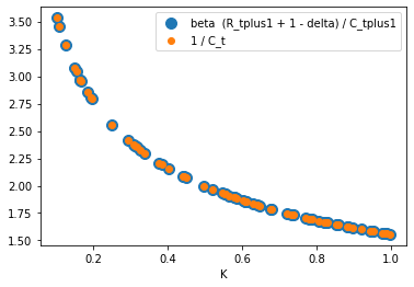
r^{\text{hand}}(K_t) = -\frac{1}{C_t} + \frac{\beta}{C_{t+1}}\,(1 - \delta + r_{t+1}).

(5)

The autodiff residual is mathematically identical. The cell below evaluates both on the same network and reports the maximum absolute difference. We expect machine-precision agreement (~10^-6 in float32).

# Hand-derived residual from notebook 01 (for verification only)
@tf.function
def euler_residual_hand(X, nn):
    K_t = X
    Y_t = K_t ** alpha
    s_t = nn(K_t)
    K_tp1 = (1.0 - delta) * K_t + Y_t * s_t
    C_t = Y_t - Y_t * s_t
    Y_tp1 = K_tp1 ** alpha
    s_tp1 = nn(K_tp1)
    C_tp1 = Y_tp1 - s_tp1 * Y_tp1
    R_tp1 = alpha * K_tp1 ** (alpha - 1.0)
    return -1.0 / C_t + beta / C_tp1 * (1.0 - delta + R_tp1)

# Compare on a grid
K_test = tf.constant(np.linspace(0.1, 1.0, 25).reshape(-1, 1), dtype=tf.float32)
res_auto = compute_cost(K_test, nn)[1]
res_hand = euler_residual_hand(K_test, nn)
max_abs_diff = tf.reduce_max(tf.abs(res_auto - res_hand)).numpy()
print(f"max | autodiff residual  -  hand-derived residual | = {max_abs_diff:.3e}")
print(f"--> They agree to machine precision; autodiff has not changed the math, only how it is computed.")

max | autodiff residual  -  hand-derived residual | = 4.768e-07
--> They agree to machine precision; autodiff has not changed the math, only how it is computed.

Sampling data¶

we make a function to generate training data. Here we just sample exogenously from an interval.

def get_training_data(k_lb, k_ub, n_data):
    X = tf.random.uniform(
    shape = [n_data, 1],
    minval=k_lb,
    maxval=k_ub,
    dtype=tf.dtypes.float32)
    return X

Training¶

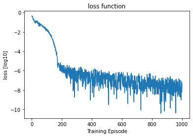
We iteratively generate training data and update the neural network

# Keep results for plotting
train_loss = []

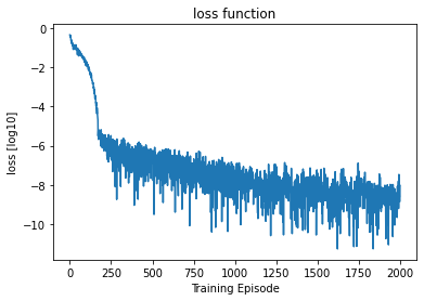
num_episodes = NUM_EPISODES
n_data_per_epi = 64
k_lb = 0.10
k_ub = 1.0


for ep in range(num_episodes):
    # generate training data
    X = get_training_data(k_lb, k_ub, n_data_per_epi)

    # compute loss and gradients
    loss, grads = grad(X, nn)
    
    # apply gradients
    optimizer.apply_gradients(zip(grads, nn.trainable_variables))
    
    # record loss
    train_loss.append(loss.numpy())
    
    # print progress
    if ep % 100 == 0:
        print("#=================================================================")
        print("episode = {}, loss [log10] = {}".format(ep, np.log10(loss.numpy())))
        
    if ep % 500 == 0:
        cost, errREE, C_t, C_tplus1, K_tplus1, R_tplus1 = compute_cost(X, nn)
        
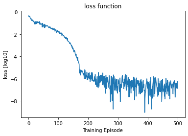
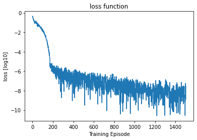
        plt.title("loss function")
        plt.plot(np.log10(np.array(train_loss)))
        plt.xlabel("Training Episode")
        plt.ylabel("loss [log10]")
        plt.show()
        plt.close()

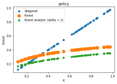
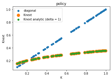
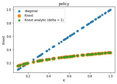
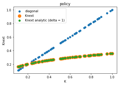
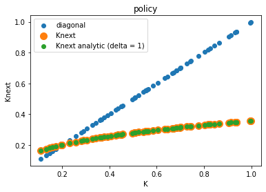
        plt.title("policy")
        plt.xlabel("K")
        plt.ylabel("Knext")
        plt.scatter(X[:, 0], X[:, 0], label = "diagonal")
        plt.scatter(X[:, 0], K_tplus1[:, 0], s=100, label = "Knext")
        plt.scatter(X[:, 0], beta * alpha * X[:, 0] ** alpha, label = "Knext analytic (delta = 1)")
        plt.legend()
        plt.show()
        plt.close()

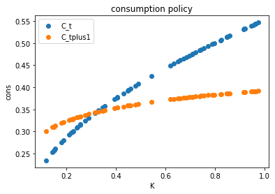
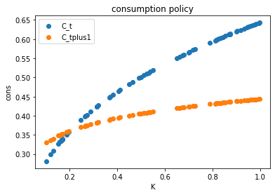
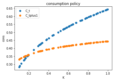
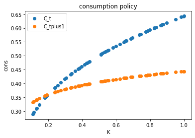
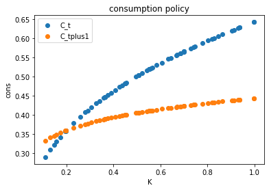
        plt.title("consumption policy")
        plt.xlabel("K")
        plt.ylabel("cons")
        plt.scatter(X[:, 0], C_t[:, 0], label="C_t")
        plt.scatter(X[:, 0], C_tplus1[:, 0], label="C_tplus1")
        plt.legend()
        plt.show()
        plt.close()

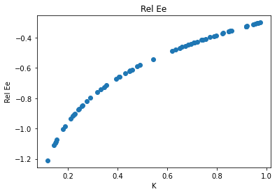
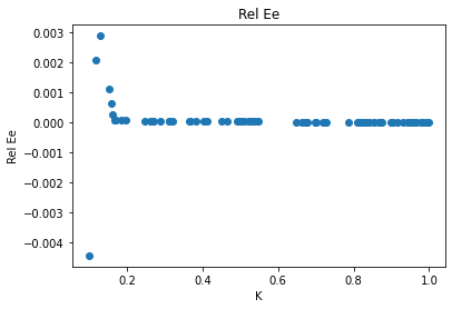
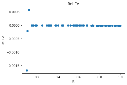
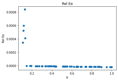
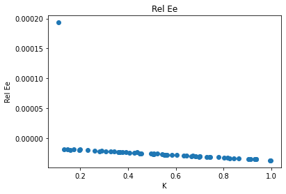
        plt.title("Rel Ee")
        plt.xlabel("K")
        plt.ylabel("Rel Ee")
        plt.scatter(X[:, 0], errREE[:, 0], label="REE")
        plt.show()
        plt.close()
       
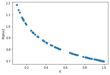
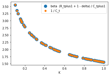
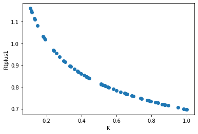
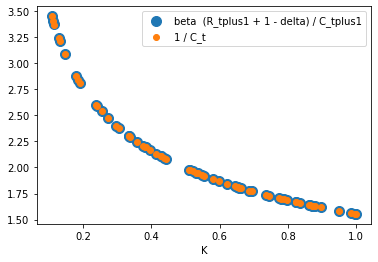
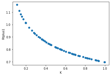
        plt.xlabel("K")
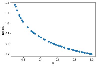
        plt.ylabel("Rtplus1")
        plt.scatter(X[:, 0], R_tplus1[:, 0], label="R_tplus1")
        plt.show()
        plt.close()

        plt.xlabel("K")
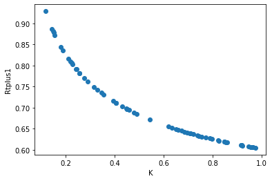
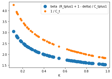
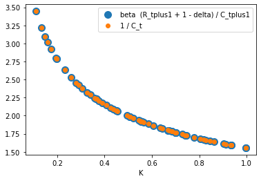
        plt.scatter(X[:, 0], beta * (R_tplus1[:, 0] + 1. - delta)/C_tplus1[:, 0], s=100, label="beta  (R_tplus1 + 1 - delta) / C_tplus1")
        plt.scatter(X[:, 0], 1/C_t[:, 0], label="1 / C_t")
        plt.legend()
        plt.show()
        plt.close()

#=================================================================
episode = 0, loss [log10] = -0.3467423617839813

#=================================================================
episode = 100, loss [log10] = -1.833279013633728

#=================================================================
episode = 200, loss [log10] = -5.5353899002075195

#=================================================================
episode = 300, loss [log10] = -6.0537872314453125

#=================================================================
episode = 400, loss [log10] = -6.268707752227783

#=================================================================
episode = 500, loss [log10] = -6.25745964050293

#=================================================================
episode = 600, loss [log10] = -6.563765048980713

#=================================================================
episode = 700, loss [log10] = -7.895870685577393

#=================================================================
episode = 800, loss [log10] = -7.621387004852295

#=================================================================
episode = 900, loss [log10] = -8.275641441345215

#=================================================================
episode = 1000, loss [log10] = -7.261270999908447

#=================================================================
episode = 1100, loss [log10] = -7.1427717208862305

#=================================================================
episode = 1200, loss [log10] = -8.71972370147705

#=================================================================
episode = 1300, loss [log10] = -8.39274787902832

#=================================================================
episode = 1400, loss [log10] = -8.43903923034668

#=================================================================
episode = 1500, loss [log10] = -7.519893646240234

#=================================================================
episode = 1600, loss [log10] = -9.657485961914062

#=================================================================
episode = 1700, loss [log10] = -7.865766525268555

#=================================================================
episode = 1800, loss [log10] = -8.601480484008789

#=================================================================
episode = 1900, loss [log10] = -8.949310302734375

#=================================================================
episode = 2000, loss [log10] = -8.824063301086426

Cross-check 2: trained policy vs the analytical solution¶

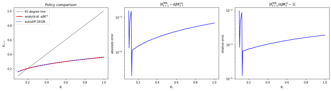
With $\delta = 1$ the closed-form planner policy is $K_{t+1} = \alpha\beta\,K_t^{\alpha}$ . We evaluate the trained network on a dense grid and report:

the policy curves overlaid (NN vs analytical),
the absolute error $|K^{\text{NN}}_{t+1} - \alpha\beta K_t^{\alpha}|$ ,
the relative error $|K^{\text{NN}}_{t+1}/\alpha\beta K_t^{\alpha} - 1|$ ,
summary statistics over the test grid.

Because the autodiff residual is the same Euler equation as in notebook 01, we expect the trained policy to match notebook 01’s accuracy.

# Analytical comparison
K_grid = tf.constant(np.linspace(k_lb, k_ub, 200).reshape(-1, 1), dtype=tf.float32)
s_grid = nn(K_grid).numpy().flatten()
K_grid_np = K_grid.numpy().flatten()
Y_grid = K_grid_np ** alpha
Kplus_nn = (1.0 - delta) * K_grid_np + Y_grid * s_grid
Kplus_an = Kplus_compute_analytic(K_grid_np, alpha, beta)

abs_err = np.abs(Kplus_nn - Kplus_an)
rel_err = abs_err / np.abs(Kplus_an)

fig, axes = plt.subplots(1, 3, figsize=(16, 4.5))

axes[0].plot(K_grid_np, K_grid_np, 'k--', lw=1, label='45-degree line')
axes[0].plot(K_grid_np, Kplus_an, 'r-', lw=2, label=r'analytical: $\alpha\beta K^{\alpha}$')
axes[0].plot(K_grid_np, Kplus_nn, 'b:', lw=2.5, label='autodiff DEQN')
axes[0].set_xlabel(r'$K_t$'); axes[0].set_ylabel(r'$K_{t+1}$')
axes[0].set_title('Policy comparison'); axes[0].legend()

axes[1].semilogy(K_grid_np, abs_err, 'b-')
axes[1].set_xlabel(r'$K_t$'); axes[1].set_ylabel('absolute error')
axes[1].set_title(r'$|K^{\rm NN}_{t+1} - \alpha\beta K_t^{\alpha}|$')

axes[2].semilogy(K_grid_np, rel_err, 'b-')
axes[2].set_xlabel(r'$K_t$'); axes[2].set_ylabel('relative error')
axes[2].set_title(r'$|K^{\rm NN}_{t+1} / \alpha\beta K_t^{\alpha} - 1|$')

plt.tight_layout(); plt.show()

print(f"Comparison on a 200-point grid in [{k_lb}, {k_ub}]:")
print(f"  max  absolute error : {abs_err.max():.3e}")
print(f"  mean absolute error : {abs_err.mean():.3e}")
print(f"  max  relative error : {rel_err.max():.3e}")
print(f"  mean relative error : {rel_err.mean():.3e}")
print(f"  steady state K_inf  : {k_infty:.6f}")
K_ss_idx = int(np.argmin(np.abs(K_grid_np - k_infty)))
print(f"  policy at K_inf     : NN -> {Kplus_nn[K_ss_idx]:.6f},  analytical -> {Kplus_an[K_ss_idx]:.6f}")

Comparison on a 200-point grid in [0.1, 1.0]:
  max  absolute error : 1.496e-05
  mean absolute error : 3.934e-06
  max  relative error : 9.616e-05
  mean relative error : 1.415e-05
  steady state K_inf  : 0.199482
  policy at K_inf     : NN -> 0.199489,  analytical -> 0.199487

Takeaway¶

We replaced two pages of pen-and-paper algebra (FOC + envelope theorem) by two tf.GradientTape calls on a single primitive Pi(K_in, K_out), where the two slots are the state and the choice.
Cross-check 1 verified that the autodiff residual is the same number as the hand-derived one (machine precision).
Cross-check 2 verified that the trained policy matches the closed-form analytical solution to comparable accuracy as notebook 01.
The pattern generalizes: any model whose period payoff can be written as $\Pi(\text{state},\text{choice})$ admits an autodiff Euler residual of the form
$\partial_2 \Pi + \beta\,\mathbb{E}[\partial_1 \Pi] = 0,$
(6)
where $\partial_2\Pi$ is the derivative in the choice slot and $\partial_1\Pi$ is the derivative in the state slot. Notebook 03 applies exactly this template to the stochastic version with AR(1) productivity.