Lecture 07, Notebook 01: Automatic Differentiation — Analytical Examples - Deep Learning for Solving and Estimating Dynamic Models in Economics and Finance

Course: Deep Learning for Solving and Estimating Dynamic Models in Economics and Finance
Script reference: §2.7.1–2.7.2 (three ways to differentiate; computational graph; forward/reverse modes), Appendix B (matrix calculus)
Notebook role: core
Author: Simon Scheidegger

RUN_MODE = "smoke"  # one of: "smoke", "teaching", "production"
SEED = 0

Automatic Differentiation: Analytical Examples¶

Notebook 1 (Day 4): companion to the autodiff lecture (deck `05b_AutoDiff_for_DEQN`)¶

This notebook accompanies the Day 4 morning lecture on automatic differentiation. It walks through six small, self-contained examples that economists will recognise:

Warm-up. A single-line autodiff demo on $y = x^2 + \sin(x)$ .
Finite differences in practice. Recreate the U-curve plot from the slides; compare against autodiff.
CRRA utility. Compute $u'(c)$ and $u''(c)$ via nested GradientTapes.
Cobb-Douglas production. A genuinely multi-variate example: marginal products $f_K, f_L$ as a 2D gradient field.
Capital adjustment cost. A second 2D example, with messy hand derivation vs one-line autodiff.
The Hessian. Second-order autodiff via a nested tape.

The two notebooks 02_Brock_Mirman_AutoDiff_DEQN and 03_Brock_Mirman_Uncertainty_AutoDiff_DEQN then apply exactly this same machinery to a full dynamic stochastic model.

import numpy as np
import tensorflow as tf
import matplotlib.pyplot as plt
plt.rcParams['font.size'] = 13

print('TensorFlow version:', tf.__version__)

2026-04-22 16:11:19.312736: E external/local_xla/xla/stream_executor/cuda/cuda_fft.cc:477] Unable to register cuFFT factory: Attempting to register factory for plugin cuFFT when one has already been registered
WARNING: All log messages before absl::InitializeLog() is called are written to STDERR
E0000 00:00:1776867079.333499   22927 cuda_dnn.cc:8310] Unable to register cuDNN factory: Attempting to register factory for plugin cuDNN when one has already been registered
E0000 00:00:1776867079.339103   22927 cuda_blas.cc:1418] Unable to register cuBLAS factory: Attempting to register factory for plugin cuBLAS when one has already been registered
2026-04-22 16:11:19.360515: I tensorflow/core/platform/cpu_feature_guard.cc:210] This TensorFlow binary is optimized to use available CPU instructions in performance-critical operations.
To enable the following instructions: AVX2 FMA, in other operations, rebuild TensorFlow with the appropriate compiler flags.

TensorFlow version: 2.18.0

1. Warm-up: $y = x^2 + \sin(x)$ ¶

Take a function whose derivative we can compute by hand:

f(x) = x^2 + \sin(x), \qquad f'(x) = 2x + \cos(x).

(1)

At $x_0 = 2$ the analytical answer is $f'(2) = 4 + \cos(2) \approx 3.5839$ .

The computer takes one line per derivative.

x = tf.Variable(2.0)

with tf.GradientTape() as tape:
    y = x**2 + tf.sin(x)

dy_dx = tape.gradient(y, x)

print(f'AD :        f\'(2)  =  {dy_dx.numpy():.10f}')
print(f'analytical: f\'(2)  =  {2*2 + np.cos(2.0):.10f}')
print(f'difference:           {abs(dy_dx.numpy() - (2*2 + np.cos(2.0))):.3e}')

AD :        f'(2)  =  3.5838532448
analytical: f'(2)  =  3.5838531635
difference:           8.133e-08

2026-04-22 16:11:22.343051: E external/local_xla/xla/stream_executor/cuda/cuda_driver.cc:152] failed call to cuInit: INTERNAL: CUDA error: Failed call to cuInit: UNKNOWN ERROR (303)

Three things to notice. (i) The tape records the forward computation. (ii) tape.gradient(y, x) walks the recorded graph backwards. (iii) The answer agrees with the closed-form derivative to machine precision -- there is no $h$ , no truncation, no roundoff.

2. Finite differences in practice¶

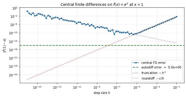
The lecture showed the theoretical U-curve. Here we plot the actual error of central finite differences applied to $f(x) = e^x$ at $x = 1$ , where $f'(1) = e \approx 2.7182818$ .

Central FD: $\widehat{f'}(x_0) = \dfrac{f(x_0 + h) - f(x_0 - h)}{2h}$ , with leading error $\tfrac{1}{6} f'''(x_0)\, h^2$ and a roundoff floor of order $\epsilon / h$ (for double precision $\epsilon \approx 10^{-16}$ ).

We will overlay the FD error against the autodiff answer.

Float precision. The next two demos cast inputs to tf.float64 so that the finite-difference U-curve and the CRRA FD comparison can show the rounding regime — in tf.float32 the rounding floor sits near 1e-6 and the U collapses. The rest of the chapter trains in tf.float32 for speed; do not carry the explicit tf.float64 casts into the DEQN training loops in notebooks 02-04.

def fd_central(f, x, h):
    return (f(x + h) - f(x - h)) / (2.0 * h)

x0 = 1.0
truth = np.exp(x0)

hs = np.logspace(-16, -1, 80)
errors = np.array([abs(fd_central(np.exp, x0, h) - truth) for h in hs])

# Autodiff answer
x_t = tf.Variable(x0, dtype=tf.float64)
with tf.GradientTape() as tape:
    y = tf.exp(x_t)
ad_err = abs(tape.gradient(y, x_t).numpy() - truth)

fig, ax = plt.subplots(figsize=(8.5, 4.5))
ax.loglog(hs, errors, 'o-', color='tab:blue', markersize=4, label='central FD error')
ax.axhline(ad_err if ad_err > 0 else 1e-16, color='tab:green', linestyle='--', linewidth=2,
           label=f'autodiff error  =  {ad_err:.1e}')
# Theoretical asymptotics
ax.loglog(hs, hs**2 * np.exp(x0) / 6, color='tab:red', linestyle=':', linewidth=1.5, label=r'truncation $\sim h^2$')
ax.loglog(hs, np.full_like(hs, 1e-16) / hs, color='tab:purple', linestyle=':', linewidth=1.5, label=r'roundoff $\sim \epsilon / h$')
ax.set_xlabel(r'step size $h$')
ax.set_ylabel(r'$|\widehat{f^\prime}(1) - e|$')
ax.set_title('Central finite differences on $f(x) = e^x$ at $x = 1$')
ax.grid(True, which='both', alpha=0.3)
ax.legend(loc='lower right', fontsize=10)
plt.tight_layout(); plt.show()

print(f'Best FD error     : {errors.min():.3e}   at h = {hs[np.argmin(errors)]:.2e}')
print(f'Autodiff error    : {ad_err:.3e}')

Best FD error     : 1.671e-11   at h = 4.29e-06
Autodiff error    : 0.000e+00

Reading the plot.

The blue dots form the classic U-curve: error first falls as $h^2$ (truncation), then climbs as $\epsilon/h$ (catastrophic cancellation).
The minimum is around $h^\star \approx \sqrt{\epsilon} \approx 10^{-5.3}$ , with best-case error $\sim 10^{-11}$ . We have lost ~5 digits.
Autodiff (green) hits machine precision at zero $h$ tuning.

For Hessians and higher derivatives, FD loses many more digits and is essentially unusable for moderate-precision work.

3. CRRA utility: $u(c) = c^{1-\gamma} / (1-\gamma)$ ¶

The standard isoelastic (CRRA) utility:

u(c) = \frac{c^{1-\gamma}}{1-\gamma}, \qquad u'(c) = c^{-\gamma}, \qquad u''(c) = -\gamma\, c^{-\gamma-1}.

(2)

We compute both derivatives via a single nested GradientTape, plot $u$ , $u'$ , $u''$ together, and confirm they match the closed-form expressions.

gamma = 2.0

def u(c):                    # the only thing we write
    return c**(1.0 - gamma) / (1.0 - gamma)

c_grid = np.linspace(0.2, 5.0, 200, dtype=np.float64)

u_vals, up_vals, upp_vals = [], [], []
for c_np in c_grid:
    c = tf.Variable(c_np, dtype=tf.float64)
    with tf.GradientTape() as t2:
        with tf.GradientTape() as t1:
            y = u(c)
        up = t1.gradient(y, c)            # first derivative via AD
    upp = t2.gradient(up, c)              # second derivative via AD
    u_vals.append(y.numpy()); up_vals.append(up.numpy()); upp_vals.append(upp.numpy())

u_vals  = np.asarray(u_vals)
up_vals = np.asarray(up_vals)
upp_vals = np.asarray(upp_vals)

# Closed-form for cross-check
up_ana  = c_grid**(-gamma)
upp_ana = -gamma * c_grid**(-gamma - 1)

print(f"max |u'(c) AD - analytical| =  {np.max(np.abs(up_vals - up_ana)):.3e}")
print(f"max |u''(c) AD - analytical| = {np.max(np.abs(upp_vals - upp_ana)):.3e}")

fig, ax = plt.subplots(figsize=(8.5, 4.7))
ax.plot(c_grid, u_vals,   label=r'$u(c)$',          linewidth=2)
ax.plot(c_grid, up_vals,  label=r"$u'(c)$ (AD)",    linewidth=2)
ax.plot(c_grid, upp_vals, label=r"$u''(c)$ (AD)",   linewidth=2)
ax.axhline(0, color='k', linewidth=0.5)
ax.set_xlabel(r'consumption $c$')
ax.set_title(rf'CRRA utility ($\gamma = {gamma}$): value, marginal, second-order')
ax.grid(True, alpha=0.3); ax.legend(loc='upper right'); plt.tight_layout(); plt.show()

max |u'(c) AD - analytical| =  0.000e+00
max |u''(c) AD - analytical| = 0.000e+00

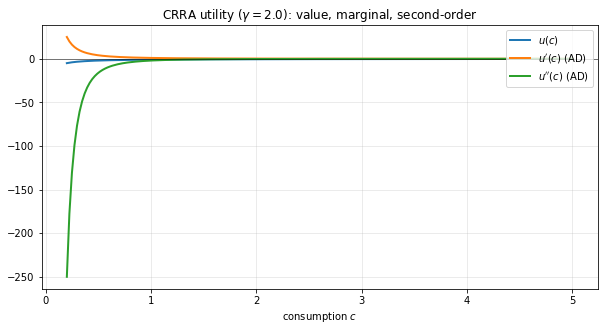
Take-away. Change gamma to 4.0 -- the code does not move. The autodiff answer follows automatically. The same cell can produce the marginal utility for any utility function we plug into u.

4. Cobb-Douglas production: a genuinely 2D example¶

f(K, L) = K^{\alpha} L^{1-\alpha}, \qquad f_K = \alpha K^{\alpha - 1} L^{1-\alpha}, \qquad f_L = (1-\alpha) K^{\alpha} L^{-\alpha}.

(3)

We will:

Compute $f$ on a 2D grid in $(K, L)$ .
Use one GradientTape to compute both partials at every grid point.
Visualise the surface and overlay the gradient field as a quiver plot.
Cross-check against the closed-form expressions.

alpha = 0.36

def f(K, L):
    return K**alpha * L**(1.0 - alpha)

# 2D grid
K_grid = np.linspace(0.5, 5.0, 25)
L_grid = np.linspace(0.5, 5.0, 25)
KK, LL = np.meshgrid(K_grid, L_grid)

# Vectorised AD on the whole grid in one go
K_t = tf.Variable(KK, dtype=tf.float64)
L_t = tf.Variable(LL, dtype=tf.float64)

with tf.GradientTape() as tape:
    Y = f(K_t, L_t)
dY = tape.gradient(Y, [K_t, L_t])
fK_ad = dY[0].numpy()
fL_ad = dY[1].numpy()

# Closed form
fK_an = alpha * KK**(alpha - 1) * LL**(1 - alpha)
fL_an = (1 - alpha) * KK**alpha * LL**(-alpha)

print(f'max |f_K (AD) - analytical| = {np.max(np.abs(fK_ad - fK_an)):.3e}')
print(f'max |f_L (AD) - analytical| = {np.max(np.abs(fL_ad - fL_an)):.3e}')

max |f_K (AD) - analytical| = 4.441e-16
max |f_L (AD) - analytical| = 1.110e-16

fig = plt.figure(figsize=(13, 5))

# Surface
ax1 = fig.add_subplot(1, 2, 1, projection='3d')
ax1.plot_surface(KK, LL, Y.numpy(), cmap='viridis', alpha=0.85, edgecolor='none')
ax1.set_xlabel(r'$K$'); ax1.set_ylabel(r'$L$'); ax1.set_zlabel(r'$f(K,L)$')
ax1.set_title(r'Cobb-Douglas surface  $K^{\alpha} L^{1-\alpha}$,  $\alpha=0.36$')

# Contour + gradient field via AD
ax2 = fig.add_subplot(1, 2, 2)
cs = ax2.contourf(KK, LL, Y.numpy(), levels=18, cmap='viridis', alpha=0.65)
plt.colorbar(cs, ax=ax2, label=r'$f(K,L)$')
# Subsample for quiver
step = 2
ax2.quiver(KK[::step,::step], LL[::step,::step],
           fK_ad[::step,::step], fL_ad[::step,::step],
           color='white', scale=15, width=0.004)
ax2.set_xlabel(r'$K$'); ax2.set_ylabel(r'$L$')
ax2.set_title(r'Contours + gradient field $\nabla f = (f_K, f_L)$ from AD')
plt.tight_layout(); plt.show()

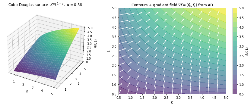
Two things this slide makes vivid.

Each white arrow is a gradient computed by autodiff at that grid point. It points in the direction of steepest increase of $f$ .
The arrows are larger near the axes (where one input is scarce, marginal product of the other is small but the imbalanced one is large) and smaller in the middle (decreasing returns). All of that behaviour falls out of one tape.gradient call; we never wrote a partial derivative.

5. Capital adjustment cost: hand vs autodiff¶

The convex adjustment cost from the Day 3 IRBC model:

\Gamma(K, K') = \frac{\kappa}{2}\, K \left(\frac{K'}{K} - 1\right)^2.

(4)

By hand: $$\frac{\partial \Gamma}{\partial K’} = \kappa \left(\frac{K’}{K} - 1\right), \qquad \frac{\partial \Gamma}{\partial K} = \frac{\kappa}{2}\left(\frac{K’}{K} - 1\right)^2

\kappa,\frac{K’}{K}\left(\frac{K’}{K} - 1\right).$$

The first one is fine. The second needs the quotient and chain rules and is exactly the kind of expression where typos hide. Autodiff: one line.

kappa = 0.3

def Gamma(K, Kp):                                         # only thing the user writes
    return 0.5 * kappa * K * (Kp / K - 1.0)**2

# 2D grid
K_grid  = np.linspace(0.5, 5.0, 30)
Kp_grid = np.linspace(0.5, 5.0, 30)
KK, KKp = np.meshgrid(K_grid, Kp_grid)

K_t  = tf.Variable(KK,  dtype=tf.float64)
Kp_t = tf.Variable(KKp, dtype=tf.float64)

with tf.GradientTape() as tape:
    G = Gamma(K_t, Kp_t)
dG = tape.gradient(G, [K_t, Kp_t])
dG_dK_ad  = dG[0].numpy()
dG_dKp_ad = dG[1].numpy()

# Hand-derived
ratio = KKp / KK
dG_dKp_an = kappa * (ratio - 1.0)
dG_dK_an  = 0.5 * kappa * (ratio - 1.0)**2 - kappa * ratio * (ratio - 1.0)

print(f"max | d Gamma/d K' (AD) - hand | = {np.max(np.abs(dG_dKp_ad - dG_dKp_an)):.3e}")
print(f"max | d Gamma/d K  (AD) - hand | = {np.max(np.abs(dG_dK_ad  - dG_dK_an )):.3e}")

max | d Gamma/d K' (AD) - hand | = 2.220e-16
max | d Gamma/d K  (AD) - hand | = 3.553e-15

fig, axes = plt.subplots(1, 2, figsize=(13, 5))

# Left: contour of Gamma + gradient quiver from AD
cs = axes[0].contourf(KK, KKp, G.numpy(), levels=18, cmap='magma', alpha=0.7)
plt.colorbar(cs, ax=axes[0], label=r'$\Gamma(K, K^\prime)$')
step = 3
axes[0].quiver(KK[::step,::step], KKp[::step,::step],
               dG_dK_ad[::step,::step], dG_dKp_ad[::step,::step],
               color='white', scale=4, width=0.005)
axes[0].plot(K_grid, K_grid, 'w--', linewidth=1.5, label=r'$K^\prime = K$  (zero adj. cost)')
axes[0].set_xlabel(r'$K$'); axes[0].set_ylabel(r'$K^\prime$')
axes[0].set_title(r'$\Gamma$ and $\nabla \Gamma$  via autodiff')
axes[0].legend(loc='upper left')

# Right: AD vs hand (cross-check)
err_K  = np.abs(dG_dK_ad  - dG_dK_an)
err_Kp = np.abs(dG_dKp_ad - dG_dKp_an)
im = axes[1].pcolormesh(KK, KKp, np.log10(err_K + err_Kp + 1e-18), shading='auto', cmap='viridis')
plt.colorbar(im, ax=axes[1], label=r'$\log_{10}\,|\nabla \Gamma_{\rm AD} - \nabla \Gamma_{\rm hand}|$')
axes[1].set_xlabel(r'$K$'); axes[1].set_ylabel(r'$K^\prime$')
axes[1].set_title('AD vs hand-derived (machine precision)')
plt.tight_layout(); plt.show()

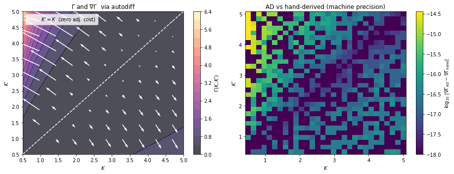
What the gradient field shows.

On the diagonal $K' = K$ , the cost is zero and $\nabla \Gamma = 0$ .
Off the diagonal, the gradient points back towards the diagonal (smoothly): the planner pays a quadratic penalty for deviating from no adjustment.

What the cross-check shows. AD agrees with the hand-derived expression to ~10^-15 across the grid. We did not have to differentiate by hand to know this is correct; we just ran both and looked at the difference.

6. Bonus: the Hessian via nested `GradientTape`¶

The Hessian of Cobb-Douglas at a point $(K, L)$ has three independent entries:

H = \begin{pmatrix} f_{KK} & f_{KL} \\ f_{KL} & f_{LL} \end{pmatrix}.

(5)

We get the whole matrix by nesting two tapes.

K = tf.Variable(3.0, dtype=tf.float64)
L = tf.Variable(2.0, dtype=tf.float64)

with tf.GradientTape() as outer:
    with tf.GradientTape() as inner:
        Y = f(K, L)
    grads = inner.gradient(Y, [K, L])
fK, fL = grads
# Now differentiate each gradient again
H_K = outer.gradient(fK, [K, L])
# Re-tape for second row (Tape is consumed)
with tf.GradientTape() as outer2:
    with tf.GradientTape() as inner2:
        Y = f(K, L)
    grads2 = inner2.gradient(Y, [K, L])
H_L = outer2.gradient(grads2[1], [K, L])

H_ad = np.array([[H_K[0].numpy(), H_K[1].numpy()],
                 [H_L[0].numpy(), H_L[1].numpy()]])

# Hand-derived Hessian
fKK = alpha * (alpha - 1) * K.numpy()**(alpha - 2) * L.numpy()**(1 - alpha)
fLL = (1 - alpha) * (-alpha) * K.numpy()**alpha * L.numpy()**(-alpha - 1)
fKL = alpha * (1 - alpha) * K.numpy()**(alpha - 1) * L.numpy()**(-alpha)
H_an = np.array([[fKK, fKL],
                 [fKL, fLL]])

print('AD Hessian:'); print(H_ad)
print('\nHand Hessian:'); print(H_an)
print(f'\nmax abs diff: {np.max(np.abs(H_ad - H_an)):.3e}')

AD Hessian:
[[-0.05924652  0.08886977]
 [ 0.08886977 -0.13330466]]

Hand Hessian:
[[-0.05924652  0.08886977]
 [ 0.08886977 -0.13330466]]

max abs diff: 1.388e-17

Three things to notice:

The Hessian is symmetric -- both AD and the hand formula recover this exactly. (AD does not assume symmetry; it gets it because it correctly computes second derivatives.)
A single nested-tape pattern generalises to any Hessian. Trying this with finite differences would lose roughly 10 digits of precision; here we lose zero.
The same idea, applied to a neural network’s loss, is what produces curvature information for second-order optimisers (K-FAC, Newton-CG, etc.).

7. Summary¶

You have just used tf.GradientTape to:

compute first and second derivatives of one-variable functions (warm-up, CRRA),
compute gradient fields on 2D grids (Cobb-Douglas, capital adjustment cost),
regenerate the textbook FD U-curve and confirm autodiff sits at machine precision,
assemble a full Hessian via two nested tapes.

In every example the user writes only the model primitive -- the utility function, the production function, the cost function. All derivatives are computed by autodiff, exactly to machine precision, with no hand algebra and no finite-difference step-size tuning.

Where to go next¶

The same pattern -- write only the period payoff $\Pi(K_t, K_{t+1}, z_t)$ , then call tape.gradient -- is what powers the Brock-Mirman DEQN solvers in:

02_Brock_Mirman_AutoDiff_DEQN.ipynb -- deterministic case; cross-checks against the analytical $K_{t+1} = \alpha\beta K_t^\alpha$ .
03_Brock_Mirman_Uncertainty_AutoDiff_DEQN.ipynb -- AR(1) productivity with Gauss-Hermite; cross-checks against the closed-form $K_{t+1} = \alpha\beta z_t K_t^\alpha$ in the full-depreciation side-experiment.

Both notebooks include numerical cross-checks of the autodiff loss against the hand-derived Euler residual at machine precision (~10^-6 in float32).

Lecture 07, Notebook 01: Automatic Differentiation — Analytical Examples