Lecture 01: Python primer

Course: Deep Learning for Solving and Estimating Dynamic Models in Economics and Finance
Script reference: Front matter (Preface, How to Read, Notation, Execution Map) and Appendix~E (Reproducibility) — Jupyter notebook orientation
Notebook role: primer (pre-course self-study; skip if you write Python every day)
Author: Simon Scheidegger

import IPython
import numpy as np
from scipy.io import wavfile
from matplotlib import pyplot as plt

Introduction to Jupyter¶

Jupyter (previously known as IPython Notebook) is an application that facilitates the development, execution, and presentation of Python code, all in one interface.
Jupyter also supports text, $\LaTeX$ , hyperlinks, images, sound files, and more.

Cells¶

A Jupyter notebook consists of seperate sections called cells. There are two main types of cells:

Markdown cells (like this cell), containing for instance text, $\LaTeX$ , or images.
Code cells, containing Python code that can be executed within the notebook.

Each code cell can be run independent of other cells, as if the code from that cell were being pasted into IPython and executed line by line.
When a cell is run, its output will be displayed directly after it.
Run the following code cell by clicking on it, holding Ctrl or Shift, and pressing Enter.
You can also click the run button (the play button) on the tool bar at the top of the page.

The top level menus expose actions along with their keyboard shortcuts.

File: actions related to files and directory
Edit: actions related to editing documents
View: actions to alter the appearance of JupyterLab
Run: actions for running code in notebooks and consoles
Kernel: actions for managing kernels (processes for running code)
Help: List of links for help on JupyterLab and kernels

Displaying websites¶

from IPython.display import IFrame
IFrame('https://www.econometricsociety.org/', 800, 400)

def factorial(n):
    """Calculate n! recursively."""
    if n < 0:
        raise ValueError("n! not defined for n < 0")
    elif n in {0, 1}:   # Base case.
        return 1
    else:               # Recursive case.
        return n * factorial(n - 1)

    
# print() displays text below the code cell.
print("3! =", factorial(3))
print("5! =", factorial(5))

# The result of the line of code at the end of the cell is displayed below the cell as output, like in IPython.
factorial(10)

3! = 6
5! = 120

3628800

The blue In [2] to the left of the cell indicates that the cell has been run, with output labeled by the red Out[2].
Once a cell has been run, all of the variables, functions, and other objects that were created in that cell are available in all other cells.
For example, the following cell has access to the factorial() function once the previous cell has been run.

print("7! =", factorial(4))

x = 50

7! = 24

Note that the above cell has no output (no Out[3] printed after the cell in red). This is because the last line of code, x = 50, does not return anything. If the cell instead ended with the code

x = 50

x

Then the output would be 50.

Now run the next cell.

x = x * 2

x

100

The output should now be 100.

Try running the previous cell again. Now it outputs 200; the value of x has been updated, even though the first time x was doubled by running the same cell. In other words, running a single cell twice executes the code in the cell twice.

⚠️ ACHTUNG! Since code cells can be run multiple times (and in any order), it is very important to be aware of which cells have been run and when.
Notebooks should be organized so that in the end, the cells can be executed sequentially without any problems. Some very hard-to-find problems can arise from executing cells multiple times or out of order.

Cells that are in the process of running, or that are waiting for another cell to finish before running, have In [*] displayed beside them. For example, run the following cell.

while True:
    x += 1

---------------------------------------------------------------------------
KeyboardInterrupt                         Traceback (most recent call last)
/tmp/ipykernel_7903/146335570.py in <module>
----> 1 while True:
      2     x += 1

KeyboardInterrupt:

At this point, Python is stuck in an infinite loop. To interrupt the loop, press the square “stop” button in the menu bar, or choose “Interrupt” from the Kernel menu. This is equivalent to pressing ctrl+c in the terminal while some code is running.

Now run the cell below to see how much x has increased during the loop.

335471564

The Kernel¶

The Python interpreter that runs notebook code under the hood is called the kernel. The Kernel menu at the top of the page has the following options.

Interrupt: stop executing code by raising a KeyboardInterrupt. Same as hitting the “stop” button in the toolbar.
Restart: stop execution and delete all variables. Every cell label goes back to In [ ], meaning none of the cells have been run yet. This is like exiting IPython, then starting it again. Same as hitting the “restart” button in the toolbar.
Restart & Clear Output: restart the kernel and delete all outputs (Out[1], figures, etc.).
Restart & Run All: restart the kernel, then run each code cell sequentially.

Try restarting the kernel by selecting Restart from the Kernel menu, or by pressing the “restart” button in the toolbar. Next, run the code cell immediately above this cell. The cell now raises an error, since restarting the kernel erased the variable x.

⚠️ ACHTUNG! Restart the kernel often to avoid using old code that was executed at one point, but was later deleted or overwritten. Then execute cells from top to bottom until you get back to where you were working.

Managing Cells¶

Running a cell with Shift and Enter moves to the next cell.
If there is no next cell, a new one is created.
To make new cells in the middle of a notebook, use the Insert menu at the top of the page or the + button in the toolbar.
The type of a cell (usually markdown or code) can be changed in the toolbar.
Try making a code cell below this markdown cell and executing some original code.
Jupyter also has many shortcuts for quick cell creation and management.
Select Keyboard Shortcuts from the Help menu for the full list.
Try the User Interface Tour from the Help menu to learn about additional features.

Images, Sounds, and Text Inline¶

Images¶

By default, matplotlib generates images in a pop-up window whenever plt.show() is called. Jupyter, on the other hand, allows graphs to be displayed between cells as an output of the code. To activate this behavior, run the code in the following cell.

%matplotlib inline
##matplotlib notebook

This command itself does not display a plot, but allows plots to be displayed inline later. Alternatively, the following command makes interactive figures inline.

%matplotlib notebook

Creating plots in Python usually requires importing modules such as numpy and matplotlib. In Jupyter it is customary to put all import statements in a single cell at the top of the notebook, like in this notebook.

Run the following cell to create a plot inline. If there is a NameError saying that the name np is not defined, run the very first cell of this notebook.

# Graph y = cos(pi*x) for x in [-2, 2].

x = np.linspace(-2,2,100)
plt.plot(x, np.cos(x*np.pi))
plt.title(r"$y = cos(\pi x)$", fontsize=18)
plt.show()     # plt.show() isn't necessary but it doesn't mess anything up.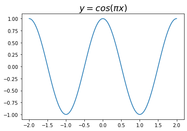

Now try making the plot interactive by changing “%matplotlib inline” to “%matplotlib notebook” two code cells ago. Re-run that cell and then re-run the cell that created the plot. Now the figure supports zooming, panning, being saved to the file system, and so on.

Sound Files¶

Jupyter can also embed sound clips in a notebook.
Start by saving a sound file in the same place as the notebook, then import the IPython module and use IPython.display.Audio() with the name of the sound file as input.
As an example, the following cell creates a short sound file called example.wav.
Then next cell embeds the sound into the notebook by creating an interactive audio bar that is connected to the sound file.

# Create example.wav, a simple sound file.
wavfile.write("example.wav", 44100, np.int16(32767 * np.sin(1000*np.pi*np.linspace(0, 10, 441000))))

# Embed example.wav into the notebook. Turn the volume down before pressing play!
IPython.display.Audio("example.wav")

Text¶

Markdown is a barebones text formatting language that allows for standard formatting like headings, italics, lists, hyperlinks, and so on. In Jupyter, markdown cells are “run” in the same way as code cells: hold shift or ctrl and press enter, or hit the “run” button in the toolbar. To edit a markdown cell, double click on it (double click on this cell, for example).

Markdown Syntax¶

Headings: Type from one to six #'s at the beginning of a line followed by a space and the heading text. The more #'s, the smaller the heading.
Italics: Surround text with one _ or one * on each side.
Bold: Surround text with two _ or two * on each side.
Hyperlinks: Surround the link text with hard brackets, followed by the URL in parentheses. For example, this link.
Lists: Start consecutive lines with a * or a - for each point in an unordered list, or with 1. 2. 3. ... in an ordered list.
Code: Surround text with one ` on each side. For code blocks, start and end with three `, followed (optionally) by the name of the language. For example,

world = None
def make_world():
    return "Hello, world!"
world = make_world()
print(world)

LaTeX¶

To embed $\LaTeX$ formatting in a Jupyter markdown cell, surround the command with either $ or $$ on each side. The single dollar sign puts it inline with the text (like this: $y = x^2 - 1$ ), and the double dollar sign centers it below the text, like the following line.

F_X(x) = \int_{-\infty}^{\infty} f_X(x) dx

(1)

⚠️ ACHTUNG! Embedding $\LaTeX$ is a feature of Jupyter, not of markdown in general.

See this page for more markdown syntax and examples.

Interactive Python¶

All of the interactive features of IPython are available in Jupyter notebook, including object introspection and tab completion.
To view the docstring for a function, module, or other object, use help, or the question mark.
A resizable help panel will appear at the bottom of the screen with the documentation.

# View the docstring about the dictionary data structure
help?
help(dict)

Help on class dict in module builtins:

class dict(object)
 |  dict() -> new empty dictionary
 |  dict(mapping) -> new dictionary initialized from a mapping object's
 |      (key, value) pairs
 |  dict(iterable) -> new dictionary initialized as if via:
 |      d = {}
 |      for k, v in iterable:
 |          d[k] = v
 |  dict(**kwargs) -> new dictionary initialized with the name=value pairs
 |      in the keyword argument list.  For example:  dict(one=1, two=2)
 |  
 |  Built-in subclasses:
 |      StgDict
 |  
 |  Methods defined here:
 |  
 |  __contains__(self, key, /)
 |      True if the dictionary has the specified key, else False.
 |  
 |  __delitem__(self, key, /)
 |      Delete self[key].
 |  
 |  __eq__(self, value, /)
 |      Return self==value.
 |  
 |  __ge__(self, value, /)
 |      Return self>=value.
 |  
 |  __getattribute__(self, name, /)
 |      Return getattr(self, name).
 |  
 |  __getitem__(...)
 |      x.__getitem__(y) <==> x[y]
 |  
 |  __gt__(self, value, /)
 |      Return self>value.
 |  
 |  __init__(self, /, *args, **kwargs)
 |      Initialize self.  See help(type(self)) for accurate signature.
 |  
 |  __ior__(self, value, /)
 |      Return self|=value.
 |  
 |  __iter__(self, /)
 |      Implement iter(self).
 |  
 |  __le__(self, value, /)
 |      Return self<=value.
 |  
 |  __len__(self, /)
 |      Return len(self).
 |  
 |  __lt__(self, value, /)
 |      Return self<value.
 |  
 |  __ne__(self, value, /)
 |      Return self!=value.
 |  
 |  __or__(self, value, /)
 |      Return self|value.
 |  
 |  __repr__(self, /)
 |      Return repr(self).
 |  
 |  __reversed__(self, /)
 |      Return a reverse iterator over the dict keys.
 |  
 |  __ror__(self, value, /)
 |      Return value|self.
 |  
 |  __setitem__(self, key, value, /)
 |      Set self[key] to value.
 |  
 |  __sizeof__(...)
 |      D.__sizeof__() -> size of D in memory, in bytes
 |  
 |  clear(...)
 |      D.clear() -> None.  Remove all items from D.
 |  
 |  copy(...)
 |      D.copy() -> a shallow copy of D
 |  
 |  get(self, key, default=None, /)
 |      Return the value for key if key is in the dictionary, else default.
 |  
 |  items(...)
 |      D.items() -> a set-like object providing a view on D's items
 |  
 |  keys(...)
 |      D.keys() -> a set-like object providing a view on D's keys
 |  
 |  pop(...)
 |      D.pop(k[,d]) -> v, remove specified key and return the corresponding value.
 |      
 |      If the key is not found, return the default if given; otherwise,
 |      raise a KeyError.
 |  
 |  popitem(self, /)
 |      Remove and return a (key, value) pair as a 2-tuple.
 |      
 |      Pairs are returned in LIFO (last-in, first-out) order.
 |      Raises KeyError if the dict is empty.
 |  
 |  setdefault(self, key, default=None, /)
 |      Insert key with a value of default if key is not in the dictionary.
 |      
 |      Return the value for key if key is in the dictionary, else default.
 |  
 |  update(...)
 |      D.update([E, ]**F) -> None.  Update D from dict/iterable E and F.
 |      If E is present and has a .keys() method, then does:  for k in E: D[k] = E[k]
 |      If E is present and lacks a .keys() method, then does:  for k, v in E: D[k] = v
 |      In either case, this is followed by: for k in F:  D[k] = F[k]
 |  
 |  values(...)
 |      D.values() -> an object providing a view on D's values
 |  
 |  ----------------------------------------------------------------------
 |  Class methods defined here:
 |  
 |  __class_getitem__(...) from builtins.type
 |      See PEP 585
 |  
 |  fromkeys(iterable, value=None, /) from builtins.type
 |      Create a new dictionary with keys from iterable and values set to value.
 |  
 |  ----------------------------------------------------------------------
 |  Static methods defined here:
 |  
 |  __new__(*args, **kwargs) from builtins.type
 |      Create and return a new object.  See help(type) for accurate signature.
 |  
 |  ----------------------------------------------------------------------
 |  Data and other attributes defined here:
 |  
 |  __hash__ = None

You can also view the attributes and methods of an object by pressing tab after typing a period after an object. Similarly, you can view what arguments a function takes by holding shift and pressing tab while the cursor is inside the paretheses of the function.

# Press tab while the cursor is at the end of the next line to view the methods of the list class.
list.

# Press shift + tab while the cursor is inside the parentheses to view argument types of list.insert().
list.insert()

  File "/tmp/ipykernel_8692/2098704207.py", line 2
    list.
         ^
SyntaxError: invalid syntax

The magic commands, or magics, are handy commands built into the IPython kernel that make it easy to perform particular tasks, for example, interacting Python’s capabilities with the operating system, another programming language, or a kernel.
IPython “magic” operations also carry over to Jupyter.
Use a single % to perform a magic operation on a single line, or use two % to perform the operation on an entire cell. The following are some of the most common and useful magics.

%lsmagic: List all available magics.
%time: Time the execution of some code.
%timeit: Execute some code several times and report the average execution time.
%prun: Run some code through the Python code profiler, printing the number of function calls and the time each takes (see the Python Essentials lab on Profiling for details).
%%bash: Run a cell with bash (as if from a terminal) in a new subprocess. Putting ! at the front of a line also triggers bash.
%%latex: Render a cell as a block of LaTeX.

# Time how long it takes to sum the integers from 1 to 100.
# Note that the sum is the cell output.
%time sum(range(101))

CPU times: user 5 µs, sys: 0 ns, total: 5 µs
Wall time: 9.3 µs

5050

# Time how long it takes to sum the squares of the integers from 1 to 100.
# Note that the sum is not reported as the cell output.
%timeit sum(i**2 for i in range(101))

20 µs ± 196 ns per loop (mean ± std. dev. of 7 runs, 10000 loops each)

%%time
# Time the execution of an entire cell
N = 1000000
current, total = 2, 0
while current < N:
    total += current
    current *= 2
print("Sum of powers of 2 less than ", N, ": ", total, sep='', end='\n\n')

Sum of powers of 2 less than 1000000: 1048574

CPU times: user 176 µs, sys: 10 µs, total: 186 µs
Wall time: 266 µs

%%bash
# This is bash, not Python.
for i in {1..3}; do
    echo $i "ah ah ah!"
done

1 ah ah ah!
2 ah ah ah!
3 ah ah ah!

%%latex
Let $A$ be an $m \times n$ matrix with columns $\{\mathbf{a}_j\}_{j=1}^n$ and entries $a_{ij}$.
If $\textbf{x}$ is a vector with entries $\{x_j\}_{j=1}^n$, then the product
$A\mathbf{x}$ is a vector $\mathbf{b}$ with entries $\{b_i\}_{i=1}^m$ satisfying
$$b_i = \sum_{j=1}^n x_j a_{ij}$$
for each $i=1,2,\ldots,m$. Furthermore,
$$\mathbf{b} = \sum_{j=1}^n x_j\mathbf{a}_j.$$

The Notebook as a Slideshow¶

Jupyter notebooks can be converted to simple slideshows.
To get started, go to “Cell Toolbar” under the View menu and select “Slideshow” (select “None” to go back to normal).
Each cell in the notebook can then be configured as one of the several kinds of slides. After selecting cell types and saving the notebook, use the following commmand in the terminal.

jupyter nbconvert [notebook_file.ipynb] --to slides --post serve

The slideshow will appear in the default browser and a file named [notebook_file].slides.html will be saved to the current directory.

# Run this cell to see this notebook as a slideshow.
!jupyter nbconvert jupyter_intro.ipynb --to slides --post serve
# Interrupt the kernel with ctrl+c to move on.

usage: jupyter [-h] [--version] [--config-dir] [--data-dir] [--runtime-dir]
               [--paths] [--json] [--debug]
               [subcommand]

Jupyter: Interactive Computing

positional arguments:
  subcommand     the subcommand to launch

options:
  -h, --help     show this help message and exit
  --version      show the versions of core jupyter packages and exit
  --config-dir   show Jupyter config dir
  --data-dir     show Jupyter data dir
  --runtime-dir  show Jupyter runtime dir
  --paths        show all Jupyter paths. Add --json for machine-readable
                 format.
  --json         output paths as machine-readable json
  --debug        output debug information about paths

Available subcommands: bundlerextension console execute migrate nbextension
notebook qtconsole serverextension troubleshoot

Jupyter command `jupyter-nbconvert` not found.

Closing Jupyter¶

Closing the browser containing a Jupyter notebook neither closes the Jupyter Notebook App nor shuts down the kernel. Instead, close the terminal that started Jupyter, or interrupt it by typing ctrl+c.

Additional Resources¶

The official Jupyter Notebook docs: http://jupyter-notebook.readthedocs.io/en/stable/
A collection of interesting Jupyter Notebooks on GitHub: https://github.com/jupyter/jupyter/wiki/A-gallery-of-interesting-Jupyter-Notebooks
Plotly’s tutorial for interactive plots in a Notebook: https://plot.ly/python/ipython-notebook-tutorial/
Project Jupyter home: http://jupyter.org
A blog on JupyterLab, the future of Jupyter notebook.